
Do:
Your goal is primarily the written report of your work. The expectation is that you'll be using various sources for your investigations, so make sure you cite all references you used: the more (that you actually use) the better. Technique, results, and presentation (especially graphics) are all important. The elegance and organization (and correctness) of the code count, but not as much as the report, which should contain enough information to convince the reader that your code must be correct.
In all this work, you will use Matlab's ODE solvers: let's just stick to ode23. The ODE solution itself is a simple and well-defined problem: one 'derivative' function just encodes the problem's differential equations (often written out for you in mathematics). The serious computing is done by a 1-liner: calling ode23 with a few simple arguments.
The non-ballistics problems can be done as a discrete set of individual experiments, each program being short and uncomplicated, basically just calls to ODE solvers. The cannon problem calls for a little interesting programming (finding the range and range-maximizing elevation with no user interaction).
A predator population of size N1 interacts with a prey population of size N2. With no predators, the prey increases exponentially by growth factor a, and with no prey, the predator population drops exponentially at rate b. Assume the number of encounters between predators and prey is proportional to a constant times the product of their populations. With constants c,d, the encounters diminish the prey population and increase the predators, respectively.
Our wolves and rabbits system is (N1 is rabbits,
N2 is wolves):
This nonlinear system is not solvable analytically, but by setting the
derivatives to zero it is easy to see that there are two equilibrium
points:
According to CSIRO studies, Australian rabbit populations multiply
8-10
times in a year (compare Fibonacci's prediction of 223 times!). Let's
say 9. Then if time units are months,
log P +12a = logP +log9
a = .1831
Average wolf lifespan in the wild is about 8 years.
If we say that 10% of wolves are still alive after 8 years, we have
Picking the rather unrealistic but round-numbered equilibrium point of 10 wolves and 100 rabbits gives d = .000240, b = .01831 .
More Realism. It would be more realistic not to allow negative-sized populations. So let's have our derivatives function set a population's value derivative dy(i) = 0 for each value of i if the value y(i) <= 0. This takes one if statement for each element of y.
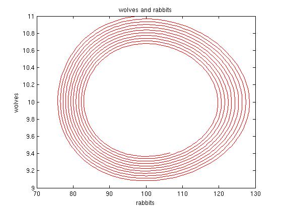
Here is the start of what happens with with an extra wolf above equilibrium (11 wolves): we can see the system heading for the equilibrium point (slowly.... this is 1000 months). That's nice, but probably not the end of the story. These systems usually wind up in limit cycles, not converging on a single point: the populations mutually wane and wax, and vice-versa, in a stable and predictable way. That means we would expect to see a stable cyclical trade-off between population species. See the exerpt from Strang's book (which you should think about owning) for the details.
The plot is a phase diagram like the Lorenz butterfly plots:
it plots
one variable against another through time. We can imagine a
point
moving through the space of variable values over time, so we visualize
the state of the system through time. This is a very common way to
display
the behavior of dynamic systems. Since this spiral is very
circle-like
we'd predict the plot of populations against time would be kind of
boring, slowly-decaying, out-of-phase sinusoids.

The control script was
y0=[100,11];
timespan = linspace(0,1000, 2000);
[T,Y] = ode23(@pred_prey_der, timespan,y0);  % all could be in one
line!
plot( Y(:,1), Y(:,2), '-r');
Assignment:
(1a) Implement the Lotka-Volterra system with Matlab's ODE solver.
Investigate the system where rabbit population multiplies at 8 times
a year, average wolf lifespan is 10 years, and the equilibrium population is
200 rabbits and 4 wolves.
Test (make and eyeball a plot or display some of the Y output
array) to make sure the system stays at
equilibrium if you set initial conditions there.
If it does, great.
(1b) In any case, start the system just a little way off equilibrium (±0.01 of a rabbit, wolf, or both, say.) When CB does this, he sees the beginnings of a spiral that gets shakier and then stops converging and just wanders around a central point in an irregular, non-repetitive circularish path.
It happens to be a (more advanced mathematical) fact that a system this size does not have chaotic solutions. So this is a good example of a computational phenomenon (present in this simulation) that mathematically can't exist, and would make you look silly if you published. Part of our job in engineering computation is having the knowledge and intuition to mistrust bogus output, and the ingenuity to understand and maybe fix it. Personal story: CB had a non-convergence issue in a physics course in 1966 but didn't recognize it, got a bad grade for the problem, and only figured out what happened years later in the middle of a grad. school numerical analysis class: finite numerical precision, duh...
In this case, we think something could be going wrong with the numerical calculation, since our previous experience and intuition tell us the solution should converge. If we knew the result about chaotic systems, that would help, but we can smell a rat without that. What to do?
From the tutorial, and from Matlab's functions and their parameters, we know that, given initial conditions, we could vary either the stepsize or the solution method. Makes sense that stepsize might be involved, since the Euler method's rectangular strips (pp 9-10 of the tutorial) fit the function better the narrower they are, and by analogy something like that must be true for higher-order methods. But if the step gets too small, close to machine precision, then we can't represent the width accurately and will lose accuracy for that reason. Matlab has a dozen built-in ODE-solvers for a reason: it makes sense that some are better for some problems, and in this case there is a higher-order (thus presumably more accurate in many cases) method, ode45, with just the same input and output parameters.
Making either change is a 5-second edit to the 3-line script that runs the solver. CB tried varying the stepsize (by changing the 3rd argument of the linspace command) up and down by several factors of two. Then he tried changing the solver function from ode23 ode45. (1c) Do a similar investigation yourself and describe what you find. Some plots would be nice.
(2) Now initialize the system to 100 rabbits and 1 wolf, and compare the phase diagram to that for 100 rabbits and 3 wolves.
(3) Man-made climate change is killing all the bunnies. Their growth
factor
According to FIGZI studies, zombie half-life is only two years since they don't floss regularly. Bad oral hygiene leads to a decay rate (hyuck, hyuck) of g = (log2)/24 = .0289. Field studies indicate that they can just get by if h = .0002, k = .0004. Zombies aren't quick enough to be great rabbit hunters, and they don't take on wolves very often since the taste is a bit gamey and those teeth can rip even more parts off: it seems that f = .002, e = .0005.
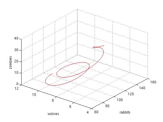
Introducing two zombies into our initial, not-quite-equilibrium situation (100 rabbits, 11 wolves with no climate change) leads to this 3-D phase diagram for 200 months...kinda interesting. One wonders if there is an equilibrium point, but consider: these equations are very much like the Lorenz attractor equations, which we know can go chaotic. Thus we should not be surprised at unpredictable-looking solutions.

The rotate tool in the figure window can be used to inspect these 3-D phase diagrams.
Assignment:
As above: implement, vary parameters,
solve, display, narrate. Make up two questions and answer them using
your
simulation.
For example: if N zombies are introduced into the system you
created in part 1, what values of h, k keep their
population stable? Likewise how can you stabilize the wolf or rabbit
populations?
Add something like the climate-change phenomenon from part 1 into the
3-species system.
Is there an initial number of wolves in, say, the part 1 situation,
that would drive zombies to zero but not kill off the wolves?
Etc., etc. Have fun, and surprise and delight us.
This exercise is mostly an opportunity to see some examples of basic natural laws that are used to formalize mathematically some simple problems chemical kinetics, or dynamic chemical reactions. A very gentle introduction to computational chemistry and chemical engineering.
Duplicate the analytically-derived solution to the Radon concentration problem (Example 3.A.4) numerically. The setup is simple, like the ball in a vacuum example in the tutorial, only here the state will simply be y (in our terms) and the derivative "vector" will simply consist of one number dy, which is not a constant, but is simply calculated from the rate constant k and y itself.
There are plenty of problems you can solve in closed form concerning the trajectory of bodies in a vacuum: Like These. But we normally fight in the atmosphere, and it turns out that air friction at muzzle-velocity speeds goes as the square of the speed of the the projectile (unlike the linear friction we saw in the mass-spring-damper example). It's also proportional to the cross-sectional area of the ball and the density of air. We get two or three coupled non-linear (because of the square of the velocity) second-order equations (for the vertical and horizontal, or also sideways, component to the ball's flight.)
Programming: Our first problem is to write the derivative functions for our problem variants. Since we want range and height of the cannonball (and later, its left-right deviation), let's say x, y, and z are the range, height, and right-deviation coordinates of the ball, respectively. Then x' (called u below), y' (called v), and z' are the x, y, and z velocity components, respectively. The physics (coming up) will give us x'', y'', and z''. That means our state vector will consist of (x, x', y, y', z, z') (in some order). The derivative function takes in the state vector and returns its derivative (it copies x', y', z' into the output and uses the physics to compute x'', y'', z'').
Physics: Let w be the ball's speed through the air (w2 = u2 + v2). A is the cross-sectional area of the ball and m its mass, ρ is the density of air (zero for a vacuum), g the force of gravity, and c is a dimensionless drag coefficient. For spheres, c tends to be about .5. Technically, c is the ratio between the actual drag force, and the theoretical drag force that would result from a hypothetical object that brought all the air it intercepted up to its own speed. Unstreamlined objects like cubes, flat surfaces normal to the airflow, and end-on cylinders tend to have drag coefficients pretty close to 1.0. Nice, streamlined, torpedo-shaped objects can have drag coefficients of 0.1 or even lower.
The force due to air resistance for a symmetrical object is directly against the direction of motion (that is, in the direction of the apparent "wind"), and has magnitude given approximately by F = (c A ρ w2) / 2. Since we are formulating the problem in terms of x, y, and x components, we have to determine the force components in those directions. In particular, we want the force in each direction as a function of of the x, y, and z velocity components (x', y' and z') Leaving z out of it for now, the unit vector in the direction of instantaneous velocity is (sina, cosa) where sina and cosa are the sin and cos of the angle of the direction of travel in the standard xy system (x horizontal, y vertical).
From F = ma, or equivalently, a = F/m we get
x'' = - (1/(2m)) (ρ c A w2 cosa) (drag alone)
y'' = -g - (1/(2m)) (ρ c A w2 sina) (gravity plus drag)
Note that we don't need to compute sines and cosines since sina and cosa can be obtained directly from the velocity vector (u,v) = (x',y'), components:
cosa = u/ √ (u2+v2)
sina = v/ √ (u2+v2)
Express the area in terms of the diameter:
a = (π d2)/4
Make all these substitutions and we have all we need to write the derivative function that computes x'' and y'' from x, x', y, y', and our physical constants.
If we choose SI units (used to be called MKS), we can choose an iron cannonball of mass 5kg: you can figure out its diameter from the density of iron: 7860 kg/m3. Air density is about 1.23 kg/m3, and g is 9.81 m/sec2.
What Now? Pick initial x0 and y0 coordinates ((0,0) makes sense) and some muzzle (initial) velocity, which should be subsonic for these equations: let's standardize on 150 m/sec, which is just under 1/2 the speed of sound. Given that and your chosen shooting elevation angle θ you can calculate the initial velocities u0 and v0 (hint: sin and cos θ are involved in the calculations).
For the problems below unless otherwise directed, use these base specifications: muzzle velocity = 150 m/s, mass of cannonball = 5kg, ρ = 1.23 kg/m3, g = 9.81, c = .5, d = diameter you figure out as above.
We have to call ode23(), and it wants the handle of the derivative function, a time span, and an initial state vector (let's say the cannon is at x = y = z = 0). Some experimentation is needed on the timespan, since our equations don't know anything about the ground and we should stop our solution about when the ball hits the ground.
With constants close to those above and
an elevation of 45 degrees I get a trajectory that looks like this: plotting
height (in m) against range (in m).
Notice the slight deviation from a pure parabola.
In fact, you can just set air
density (ρ) to 0 and run that case with
>> hold on
to superimpose the plots and see a dramatic range difference.
Soon you'll be asked to see how elevation,
drag, and mass affect the trajectory.
You'd expect a lighter, projectile to slow down faster
(from intuition, maybe, but preferably from the equations!).
So it would have a more asymmetric trajectory.
 .
.
Footnote:
Who's this kindly old gentleman?
 (from wikimedia commons, Scanned from German "Meyer's Encyclopedia",
1906.)
Turns out for
modern bullets there's a special drag coefficient called the
The
Ballistic Coefficient . It is a number based on
the drag coefficient, only normalized to an "ideal bullet"
that this
benign duffer produced in 1881, with ballistic coefficient of 1 by
definition. (So now you know: if he's dictating standards, he's
not just somebody's beloved grandpa).
Unlike the drag coefficient, a smaller ballistic coefficient means more drag.
Regular bullets in use today have ballistic coefs varying from
about .01 (.177
pellets)
to about 1, but you can make a bullet with BC 1.1 out of special
materials with special lathes...better than the first "ideal bullet".
 .
.
Battle of Crécy between the English and French in the Hundred Years' War. From a 15th-century illuminated manuscript of Jean Froissart's Chronicles (BNF, FR 2643, fol. 165v). (Commons.Wikimedia.org)
FWIW, I get a pretty significant deflection in z for the base specifications and 45 degree shooting angle.
Code To Write:
function dy = cannon_der(t,y)
script shoot.m
function x0 = zero_cross(x,y)
function x = range(angle, diameter, mass)
function xmax = max_range(low_angle, high_angle)
function dy = cannon_air_der(t,y)
function dy = cannon_der(t,y) This is the always-needed derivative equations whose handle you pass to your ODE solver. It specifies the derivatives for the state vector that consists, in some order that makes sense to you, of the quantities (x,y,z,x',y',z'). The output is a COLUMN 6-vector specifying their derivatives (x', y', z', x'', y'', z''). The z (East-West) direction is used in the last part of the question. Note that since there is no explicit time dependence in this problem, the t value will be ignored. It is needed only to fit the form used by ode23().
script shoot.m This is simply the call to ode23() and various plot commands to help get acquainted with the problem and for parts 1 and 5 of the assignment.
function x = range(der_func_handle, angle, diameter, mass) This is the basic cannon-shooting simulator that we can use in all parts of the assignment. It uses your ODE solver (ode23() is fine) to compute the range of the cannonball (where its height (y) goes to 0). Thus this function needs the handle to cannon_der, it needs to set initial conditions (using the angle) and a time span (experiment until you get one that gets y (height) into negative values for the range of angles you want to consider) and it calls zero-cross. Its parameters are the most commonly-changed ones (and you have to change them in the second part of the assignment).
IMPORTANT! cannon_der() needs to use these parameters (angle, diameter, mass) but we can't pass them into cannon_der() since its parameters have to look like (t,y). So declare these variables global in both cannon_der() and range().
function x0 = zero_cross(x,y) processes the output of ode23() to estimate the value of x for which the ball hits the ground (i.e. for which y(x) = 0). ode23's output consists of the varying state vector Y (each row is a [x y z x' y' z'] vector) and the associated x value vector, where Y = f(x). x0 is the computed estimate of the value of x for which y=0. One coarse estimate is the first x for which y changes sign from positive to negative.
Better is a linear interpolation: Let's say y starts out positive, as in this assignment. Given (x1,y1), with y1 the last positive y, and its neighboring point (x2,y2), with y2 the first negative y, you can draw a little picture with the two points, a line between them, and the line y=0, and notice you want to solve for x0, where a point on the line is (x0,0). A similar triangles argument and a little high school algebra gives you x0 in terms of x1, y1, x2, and y2.
function xmax = max_range(low_angle, high_angle) This answers the second part of the assignment. It calls range() for various angles (maybe let them vary freom low to high by 2 degrees?), gets the ranges and returns the maximum one. I'd use a single for-loop that initializes a variable max_range to the first range and best_angle to the first angle, and subsequently updates the max_range and best_angle to the current range and angle if the current range is longer than the previous max.
function dy = cannon_air_der(t,y) For the fourth part, we need a new derivative function that is just like cannon_der (globals and all) but instead of being a constant, the air-density is a function of ρ, the sea-level density, and y (the height). That change must be made in the three derivative functions for x', y', and z'. Come up with a close-enough function (e.g. google 'air density table'), justify it with a reference, and carry on!
The NYTimes has hired us to quantify (and thereby they hope to invalidate) their right-wing rival's story. Here's what we (well, you) will do. (Note: NYTimes needs references for all numbers, functions, facts, etc.). About 10 minutes googling should be all you need too.
The strategy is to simulate the trajectories of hits, see if each hint is a homer, and to see if we can replicate the claimed statistical improvement in the number of homers given different velocities of following winds.
Hint: don't even think about writing your final program and starting to play with it. Small routines, thoroughly understood and debugged: that's the thing. For instance, you could test your monte carlo routine by only varying one parameter (elevation or velocity), using a simple uniform distribution, and making sure the data make sense). Then the other parameter. Only then do both. Continue this conservative approach.
All this is used in a Monte Carlo simulation to generate a realistic population of ball trajectories. Monte Carlo is just a fancy way of saying "repeated probabilistic simulation": A simpler example is the way π was used in Ass't 5, π part 3, Monte Carlo .
You'll want to discard numbers below and above some thresholds (velocity should be between some reasonable minimum speed off the bat (40 mph?) and some known maximum whose value you can get from the web.
Do your results, given the limittions of your approximations, agree with the story?
If that link dies, here's a local copy. Offhand, what do you think of his science? Present your data on the downward angle and compare. How does our W-b E's assumptions with your findings.
See the Universal Hand-In Guide.
Briefly, for the Code component of this assignment, you'll need a .zip (not .rar) archive with code files and README.
Submit the writeup as a single, non-zipped .PDF file. Submit before the drop-dead date for any credit and before the due date for partial-to-full (or extra!) credit.
Check immediately to see BB got what you sent!