Randomized Algorithms

Weiss Ch. 10.4.

Randomized Algorithms are an important subspeciality. They are quite important practically, and came to prominence recently in cryptography.

The Evil Professor's Unpredictable SFS scheduling is an example from the text. With positive reinforcement, the random schedules and amounts of rewards makes for quicker learning and longer perseverance. A poker player (say a computer) who has no tells and bluffs and sandbags randomly forces his opponent to abandon psychology and descend to basic odds.

The random patterns found in wildlife make for unpredictable, rarely-reproduced behavior that actually does not come natural to humans. Prey species naturally make life hard for predators, but humans sometimes need security consultants to enforce random behavior.

Enough biology. The text considers briefly a randomized quicksort (choose a random list element as pivot vs. always choosing the first element), which has O(N log N) expected-time behavior and is not subject to the predictable problems of choosing first element as pivot (e.g. almost-sorted inputs,) even though both approaches have worst-case behavior of O(N².

With randomized algorithms, there are no bad inputs (a sorted list is always bad for the choose-first-element pivoting strategy). There are "bad random numbers" (a.k.a. bad luck) -- e.g. the random pivot could be smallest element of the list every time...)

Randomized algorithms yield expected running time for any input. E.g. the random-pivot quicksort has expected time O(NlogN) for both a sorted list and a random list.

We skipped over them pretty fast, but we saw randomized algorithms in perfect and universal hashing.

We'll spend most of our time on the idea, which has applications beyond cryptography, called Monte Carlo (and Las Vegas) algorithms.

(Pseudo) Random Number Generators

Weiss 10.4.1

By definition, an algorithm can't produce random numbers, though generators for crypto and other critical applications are not only more sophisticated mathematically, but often are interactive and use many statistics from "the world" (like disk access times, process numbers, machine load factors, user typing statistics, time of day, etc etc.).

Typically applications want a stream of uniformly-distributed, random-looking reals or ints in some range. From them other distributions like Gaussian, Poisson, etc. can be built. Also we may want to "replay" the random sequence to check for algorithmic repeatability, so a user-provided seed is often an optional feature, as are a range of more or less efficient generators.

Lots is known about pseudo-random generators, but there are still weak ones out there in common compilers (cf. Weiss). Text- and reference-book literature goes back to Knuth, who among other things noticed that combining a lot of random number generators actually generated worse results. Also Knuth analyzes the generators known at time of writing (early 1970's).

Weiss tells us about linear congruential generators, which go back to the 1950's and which are fine for everyday use: the idea is to compute a sequence from a seed x₀ by

If A and M are chosen with care the sequence repeats only after M-1 numbers. If M is prime, they are non zero. A good pair of numbers known to Lehmer ('51) is:
M = 2³¹ -1 = 2,147,483,647
A = 48,271.

"...with random number generators, tinkering usually means breaking..." (Weiss p. 477).
E.g.

just (re)generates the seed 179,424,105.

Naive implementation runs into problems with overflow that affect the random properties. Easy to fix -- if the new random number (and state) overflows and thus evaluates to a negative number, just add M to it (Fig. 10.55).

"Surely we just leave all this to the compiler and math library!?" Nope, lots of libraries (thus languages) use versions of xi+1 = (Axi +C) mod 2B, with B the number of bits in an integer. Clearly that mod 2^B should be a big red flag. In fact it makes last bit of x_i alternate beween 0 and 1 (even, odd, even, odd...) (!!). Clearly, and likewise the low order k bits form a cycle of length 2^k (!!). Java and unix's drand48 use a 48 bit linear congruential generator but return only the high 32 bits, so eliminating short cycles but leaving long ones that could appear in big experiments.

MAW (Fig 10-56) gives and explains a 48-bit generator using Java's 64-bit capabilities that has better properties than the 31-bit one above.

Skip List Driveby

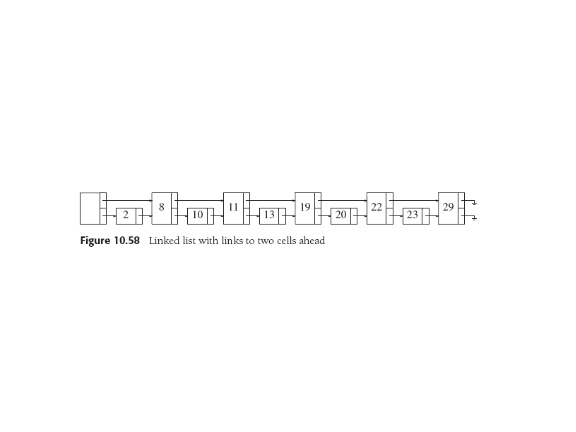
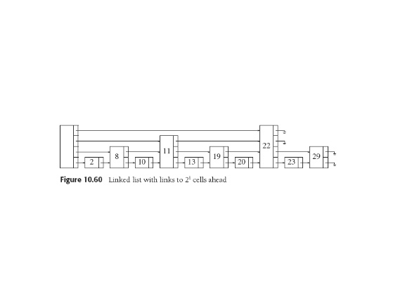
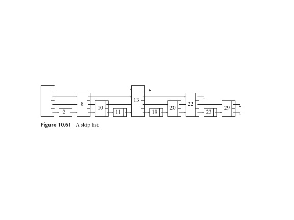
Weiss 10.4.2: As in hashing, need to know approximate number of items N to pick a maximum height logN. Idea should be obvious, and should obviously imply (logN) insertion and delete.

To search: start at highest link in header, follow that level until find next node is larger than the one we're looking for or null. Then drop to next lower level and continue. When get to level one, node we seek is next or not there.

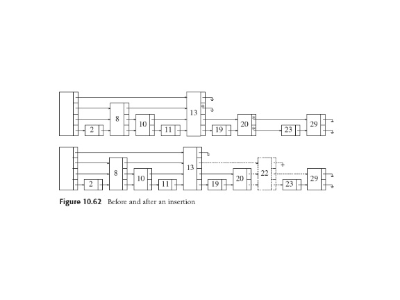
For insertion, search while marking points we drop a level. Use repeated coin-flipping technique to find height H such that prob(H) = 1/2^H. Thus maintain random distribution of node heights, and the O(logN) lookup and insertion times.

(Pseudo) Primality Testing and Monte Carlo Algorithms

Weiss 10.4.3

Really it's "compositeness testing". Became critical with public key crypto, which needs large (200 digit?) primes. Naive testing for N is to try dividing N by every prime up to √N. Easiest implementation is to divide by every odd number between 3 and √N, which is about √N/2 divisions. Now if d is the number of digits in N and we need d=200 say, then we'll need 10¹⁰⁰ divisions: gulp.

Monte Carlo and Las Vegas algorithms (see Wikipedia, Randomized Algorithms) are not the same as Monte Carlo simulations. Suppose we have an algorithm to answer a question that responds probabilistically every time it's run. Given a composite input, half the time (provably half the time) it says "Definitely not" (for us, "composite!, definitely not prime"), and half the time "Maybe so, maybe no, I dunno" (possibly prime).

Now when it says "not", it has a counter-example. The answer is really, truly no. So if the algorithm's internal "trials" are independent, and it answers "maybe" 20 times, then that's 20 times it couldn't find a counter-example, which could only happen at random one time in a million (2²⁰) if the number is composite, but is consistent with it being prime.

So even with no definite proof of primality, the probability the answer is "composite" is small now, and if the answer really is "composite", that probability will only get smaller with more tests.

Fermat's Little Theorem

A good primality test is based on FLT.

FLT is:
If P prime, 0 < A < P, then A^P ≡ A (mod P).
Equivalently:
If P prime, 0 < A < P, then A^P-1 ≡ 1 (mod P).

There are enough proofs of FLT to have their own Wikipedia page, which is worth looking over. The binomial-coefficient proof is nice and the group theory one's a 4-liner (power of abstraction). I like this easy combinatorics one, attributed to Golumb.

Plan is to divide A^P things into two sets that account for them all. The first set will have A things in it, and the second will have a whole number n of subsets, each of which is P long. Thus A^P = nP +A, which implies the theorem.

A^P counts the number of P-long sequences of A values, the first sort of counting we did in combinatorics. So for example there are 2⁸ eight-bit bites. If A is 3, not two, we're in trinary numbers, if A is 10 we've got decimal, etc. We'll use binary here but notice it's without loss of generality.

With P prime, a P-long sequence has no repeated subsequences: a 6-long number can be 110110 or 101010, which look the same after a rotation of 3 and 2 or 4, respectively, since 6 has factors 2 and 3. With no factors, there are no repeated subsequences that take up the whole sequence.

Let's consider A=2, P = 5 as our example. You can't make a 5-long binary number (generally P-long A-ary number) that's the same upon rotation. Or can you?

Right: 11111 and 00000. So with P prime, There are A of these special numbers in general, (2 for A=2). That leaves 30 in the example. Let's enumerate them: plan is to pick one, generate its rotations, which had better be all different, and of which there will be exactly 5, then find any number not yet generated and rotate it, etc.

start    rotated values
          in decimal
00001    1  2  4  8 16
00011    3  6 12 24 17
00101    5 10 20  9 18
00111    7 14 28 25 19
01011   11 22 13 26 21
01111   15 30 29 27 23 

Indeed. We eat up P at a time, they can't repeat within the row by P-prime argument above, if we pick a new one its row can never contain a number in any other row else the whole row would be the same, and each row has to have P entries.

Therefore we get A sequences that are just repetititions of each value of A (eg for ternary, 000..., 111..., 222...). Then we have the n rows each with P rotated entries, for some integer n.
So A^P = nP +A, QED.

The table of rotated values has a little structure, but it's hazy: in fact each row shows a mini-congruential generator; some have bad choices of seed and all have A=2, so the randomness past row 1 is actually pretty striking.

FLT as Composite (non-Prime) Test

Simple. You give me an N to check for primality. For FLT, I must compute A^N-1 for some A (like 2). How do we implement the exponentiation to the (possibly huge) N? Use the pow efficient exponentiation algorithm from 2.4.4. So the FLT test is computationally possible O(logN) using pow (Weiss Fig. 2.11, p. 48).

By FLT, if A^N-1 is not ≡ 1 (mod P), we're certain N is not prime. If answer ≡ 1 (mod P) it probably is. (e.g. 341 is the first N that fails this test for A=2). And if we pick A = 3, 341 is shown composite). Now there are certain numbers (Carmichael Numbers) that are not prime but satisfy our condition for all A < N that are relatively prime to N. Smallest is 561. We need another test! Weiss's Theorem 10.11, (related to a result we saw in quadratic hashing) is used in the algorithm Fig. 10.63.

The well-known Miller-Rabin primality test likewise uses another easy-to-check number-theoretic property and applies it at every stage of the exponentiation process. Weiss's version seems easier to me.

Miller-Rabin a la Weiss

Back in Ch. 5.1 p. 182 we were looking at properties of quadratic hashing and proved something about i² (mod P) for prime table sizes. Now this...

If P prime and 0 < X < P,
the only solutions to X² ≡ 1 (mod P) are
X= 1 or X = P-1.

Proof: If X² ≡ 1 (mod P) then
X² -1 ≡ 0 (mod P), so
(X-1)(X+1) ≡ 0 (mod P).

Thus, with P prime and 0 < X < P,
P must divide either (X-1) or (X+1)
and we're done.
e.g. nP = (X-1) implies X = 1.

We check this property of A^N-1 at every stage of the FLT exponentiation process in our FLT test (last overhead). If A fails the test then N is composite, guaranteed. But what if N is not prime? Well, the test can be fooled (it's an "if" not an "only if"). But it's provable that for large N at most (N-9)/4 values of A fool the algorithm. And these worst cases are much rarer than N/4.

So if A chosen at random and the algorithm does not flunk N out, chances are (better than) about 3/4 that N is really prime. With probability of non-primeness dropping by factor of four per trial, the probabiliby a non-prime will fool the algorithm in 50 independent trials is < 2^-100.

Weiss gives us the complete code in Fig. 10.63. One of my crypto books shows M-R working on N= 561, the pesky Carmichal number.

If N is composite but passes FLT test A^N-1 ≡ 1 (mod N), it is a pseudoprime for the base A. If it also passes the Miller-Rabin test, it is a strong pseudoprime for the base A. There are 455,052,511 primes less than 10¹⁰ with 14884 pseudoprimes and 3291 strong pseudoprimes for base (that is, A = ) 2.

In last paragraph Weiss points to work on deterministic polynomial time primality tests. Stay tuned, the NSA is very interested!