
Tree Overview
Weiss Ch. 4.1 - 4.
Trees' ubiquity and utility: expression and evaluation (parse trees,
expression trees), dictionaries for O(logN) search, insertion,
deletion. Binary and k-ary trees.
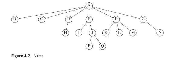
Definitions
Many definitions, most analogous to Western family relationships,
except for the root and leaves.
CS Trees are notoriously recursive in structure, so the "branches" are
called subtrees.

Path between nodes is the sequence of nodes leading (through
successors or children) from one to the other; its length is the
number of nodes - 1, so node has 0-length path to self. Depth of node
is length of unique path (else it's a graph) from
root. Height of a node is length of longest path from it to a
leaf. Height of empty tree is -1.
Implementations
There are some cute tree implementations that use arrays (e.g. full
binary trees), but generally think of structures (classes) and
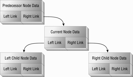
pointers. For k-ary trees with small k, works to have pointers to
explicit (left, middle, right...) children in the node, but an easy
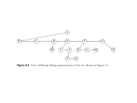
extension to deal with arbitrary numbers of children is the "first
child, next sibling" implementation (fig. 4.4), in which each's nodes children
are in a linked list.
Binary Tree More Explicitly:
Binary Tree Java:

Tree Traversals W 4.1.2
A rooted tree has only one root, but really
trees have sub-trees that look just like trees. They are thus naturals
for recursive techniques and arguments.
So: To traverse (visit all nodes in) tree, first visit the root, then
visit all the children. Or vice-versa. (pseudocode Fig. 4.6).
We need to see that visiting the root is not the same as visiting the
children. The first (root) is the recursion-ending base case, and the
second
(child) is a recursive call that descends a recursive level. Also
"visit"
is short for "do necessary work on".
With binary trees, there are three common and useful O(N) recursive
methods: Preorder (do root, do left child, do right child), Inorder
(left, root, right), and postorder (left, right, root). For the perverse,
inverting left and right gives more traversals.
Preorder allows a
natural way to list files in a UNIX directory -- UNIX directory also has
. and .., (self- and back-pointers)
so not a pure tree. To get cumulative disk usage we
need postorder. To compute the height of each node also need
postorder.
Another sometimes-useful traversal is level-order,
which lists all nodes at depth 0, 1, 2, 3....and works iteratively with
a queue of children to print.
Binary Trees: Expressions W 4.2
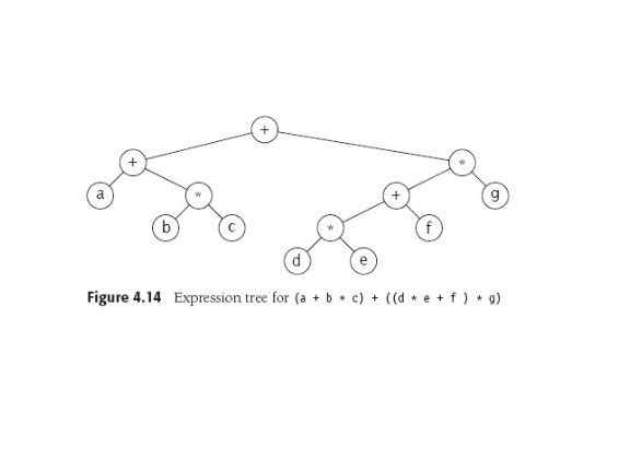
W. 4.2.2 introduces shows expression trees (see also the relevant
lecture PPTs),
which are a natural notation for
arithmetic expressions and can be traversed by inorder -- produce
parenthesized expression of left subtree, then emit the operator, then
the parenthesized expr. for right subtree. Or can print out (left,
right, operator -- postorder) and get postfix notation out, or a
preorder
traversal gives a polish prefix expression.
Or can traverse (inorder most natural) to evaluate the expression and get an
answer.
Construction of a tree from a postfix expression is just like
evaluation of the postfix using a stack. Look one char at a time, if
it's an operand then make a
one-node tree and put it on stack, if an operator, pop two trees and make
a new tree.
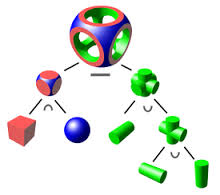
Constructive Solid Geometry (CSG) 3-D models. leaves are
primitive solids, internal nodes are set operators. Ray casting and
Boundary evaluation. Hardware implementation.
The Idea:
 In Practice (POV-Ray)

Binary Trees: Search Tree ADT
Don't want to do linear search through an array or list to locate an
item. Hence trees: ideally need log(N) levels for N items, so maximum
path to any item is log(N).
Make sure you understand last sentence. Balanced (full, ideal) Binary Trees: N elts at one level means 2N
at next level, so with k levels (∑k 2k) -1
elts in tree (1, 3, 7, 15,...), add one to each and thus show
the depth is (just) > the log of the number of elts.
BUT naive methods for inserting and
deleting can yield trees with O(N) path-lengths (e.g. no right children).
Hence the interesting insertion and deletion algorithms
that have been created by smart people over decades...
Weiss fig. 4.17 shows his ADT for trees: the most basic functionality
is
insert and : also we've got: print,
contains (a
boolean), min, max
(for trees of comparable elts), makeEmpty, isEmpty.
Weiss discusses his code for all this at length with us: nice
fireside chat --- mighty relaxin'. 113-120. Along the way, salient
points about duplicates, fact that in data structures deletes are
often harder than inserts, lazy deletion, other nuggets.
Binary Search Trees: Some Details
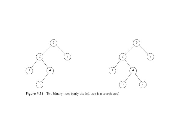
In a BST, for any node X, all the items in X's left subtree are
smaller than X and all those in its right subtree are larger. The
obvious way to find something that's not the current node is:
want smaller, visit left subtree;
want larger, visit right.
The BST
property is
not
local to a node and its children:
Contains: Need to test nodes: if null, return false (not there); if
equal to desired, return true.
Else
recursively call contains on L or R subtree depending on comparison. Note
these are tail-recursive calls so can be replaced by while loops!
FindMin, FindMax: go all the way down to left or right. Recursively
or iteratively.
Insert X: Proceed as for Contains: if find X, do what you want about
duplicates; otherwise insert X at last spot traversed. (fig. 4.21)
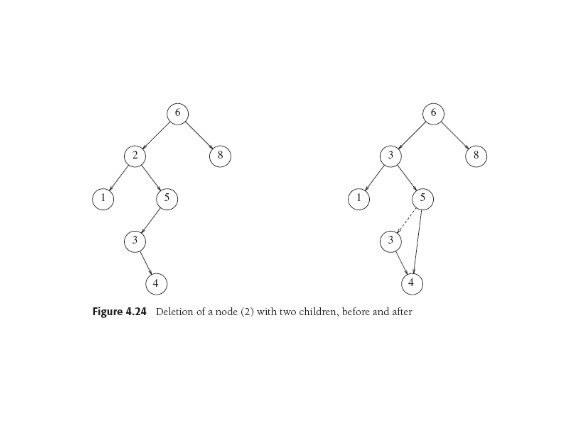
Delete X; Easy if node is leaf or has only one child. Two children:
replace with smallest value in right subtree, which gets deleted (and
it only can have one child or it wouldn't be smallest, right?).
Analyis: Ave. Case and Recurrence
W. 4.3.5 is quite a fun little section. For BSTs, average case
analysis is possible -- a rare treat.
We can characterize useful tree statistics if all insertion sequences
are equally
likely.
The relevant statistic for search is the average (hence the total) path length in
a tree; called its internal path length D(N).
The math of the analysis points ahead to recurrence equations,
which we'll deal with later. For now, read this little section
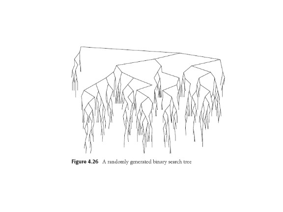
"for pleasure". The two figures illustrate a probably
"unintended consequence" (nasty surprise) of the delete algorithm.
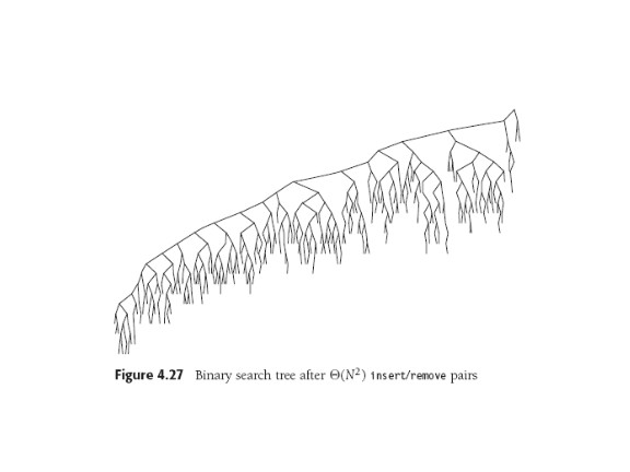 Can you explain the problem?
Motivation to Keep On...
Properties of simple BSTs motivate the two approaches:
1: being careful
to construct and maintain balance in the tree (e.g. AVL trees,
red-black trees, 2-3 trees...) to
guarantee logN lookup every time. Clever algorithms, tougher
implementations.
OR
2: to guarantee no sequence of long (O(N)) lookups can happen by
modifying ("self-adjusting") the tree upon each lookup (e.g. promoting whoever's found to be
the new root!): Splay trees. This idea aims at good
amortized
(averaged over time)
performance (since each bad case leads to immediate
improvement).

Last update: 7/15/13


 In Practice (POV-Ray)


 Can you explain the problem?
