SALT: Symbolic Analysis of Loop Tiling

Yanghui Wu ywu86@ur.rochester.edu

Yifan Zhu yifanzhu@rochester.edu

Yekai Pan ypan34@u.rochester.edu

Chen Ding cding@cs.rochester.edu

University of Rochester
Rochester, NY
USA

DOI: https://doi.org/10.1145/3838684.3846873
PACT '26: International Conference on Parallel Architectures and Compilation Techniques, Chicago, IL, USA, October 2026

Loop tiling is central to compiler optimization, yet predicting its cache behavior remains difficult because problem dimensions, tile sizes, tiling depth, cache capacity, and block size interact. Existing techniques typically fix some of these parameters or analyze loop structure and cache behavior separately.

This paper presents SALT, a compiler technique for deriving approximate parametric cache miss ratios for symbolically bounded rectangular loop nests with affine array accesses. SALT maps each static array reference to a reuse-interval distribution and applies Denning's working-set recursion to construct a parametric miss-ratio curve for a fully associative LRU cache. It supports untiled and multilevel rectangularly tiled kernels, including matrix multiplication, tensor contractions, and stencils. The analysis is fully static, keeps program, tiling, and cache parameters symbolic, and does not enumerate concrete values; instead, its cost depends on the product of loop depth and the number of static memory references.

We implement SALT in Rust within an MLIR-based toolchain and evaluate it on tiled and untiled kernels. Its predictions closely match cache simulation and achieve a mean absolute percentage error of $1.68 %$ across the hardware-counter validation experiments. Across eight tensor kernels, SALT is approximately 78 × faster than our polyhedral counting baseline, implemented using Barvinok, and 11, 000 × faster than Cachegrind simulation, making its analysis practical to integrate into a compiler.

CCS Concepts: • Theory of computation → Program analysis; • Software and its engineering → Compilers; • Computing methodologies → Symbolic and algebraic algorithms; • Computer systems organization → Processors and memory architectures; Software performance;

Keywords: symbolic cache analysis, cache locality, reuse intervals, cache performance modeling, loop tiling

ACM Reference Format:
Yanghui Wu, Yifan Zhu, Yekai Pan, and Chen Ding. 2026. SALT: Symbolic Analysis of Loop Tiling. In International Conference on Parallel Architectures and Compilation Techniques (PACT '26), October 19--22, 2026, Chicago, IL, USA. ACM, New York, NY, USA 13 Pages. https://doi.org/10.1145/3838684.3846873

1 Introduction

Tiling is an important loop transformation in modern compilers [1, 2, 3, 42], transformation frameworks [31, 45], and domain-specific languages and compilers for image processing [33] and tensor operations [23, 27, 36].

While the practical benefits of loop tiling are well documented, its effect on cache behavior is difficult to analyze statically. Tiling changes the reuse structure of a loop nest, but cache performance depends on how reuse interacts with cache capacity, cache block size, and dynamic cache replacement.

Existing reuse-distance and cache-prediction models are generally trace-based, online, or hardware-assisted. They establish reuse distributions for fixed program instances or tiling configurations, but they do not provide a fully static symbolic derivation of those distributions from loop code. Standard affine analysis handles more general polyhedral iteration spaces. In contrast, SALT targets rectangular loop nests and directly supports symbolic forms introduced by tiling, including symbolic strides, products between tile parameters and loop indices, and quotients such as n/t. SALT also handles expressions involving symbolic cache block size; Section 2.2 gives the precise input scope and limitations.

This paper presents Symbolic Analysis of Loop Tiling (SALT), a compiler technique that derives parametric cache miss-ratio expressions for symbolically bounded rectangular loop nests with affine array accesses. This target class includes both untiled affine kernels and kernels produced by any number of rectangular tiling levels. SALT treats tiling uniformly as additional loop levels and symbolic trip counts rather than as a separate input form. It keeps problem dimensions, loop bounds, applicable tiling parameters, cache capacity, and cache block size symbolic under a fully associative LRU cache model.

SALT proceeds in three steps. First, it maps each static array reference to a reference access vector that records how the loop indices participate in its subscripts. Second, it derives the reference's temporal and spatial reuse-interval distribution; for stencil-style references, SALT also handles restricted constant-offset group reuse. Third, it applies Denning recursion to convert the distribution into an approximate symbolic cache miss-ratio expression. The analysis runs in time proportional to the product of the number of loop indices and the number of static memory references.

General Presburger arithmetic techniques can model more general affine iteration spaces, including index-dependent bounds and affine conditionals. However, they cannot directly express multiplication between variables or division by symbolic terms [4, 5, 16, 18, 22, 32]. SALT makes a complementary tradeoff: it specializes to rectangular iteration spaces with loop-invariant symbolic bounds. In this domain, SALT retains problem sizes, tile sizes (when present), and cache block size when they occur as symbolic strides, coefficients, or divisors. Complementary algorithmic studies derive asymptotic I/O bounds for local memory, either with explicit data movement or with a cache [14, 15, 20, 30].

The main contributions of this paper are as follows:

A new symbolic method (SALT) that derives reuse-interval distributions and approximate parametric cache miss-ratio expressions for symbolically bounded rectangular loop nests with affine array accesses, including untiled and multilevel-tiled kernels.
A compiler implementation in an MLIR-based toolchain [26] using the Symbolica library for polynomial arithmetic.
An experimental evaluation using matrix multiplication and eight tensor kernels, comparing SALT with cache simulation and a Barvinok-based polyhedral counting baseline, together with hardware-counter validation on the tensor kernels and a 5-point stencil.

As matrix multiplication is transformed from untiled to two-level tiled code, our Barvinok-based polyhedral baseline slows from 0.17 seconds to 89.2 seconds, while simulation takes between approximately 1 minute and 46 minutes across the evaluated configurations and input sizes. SALT requires milliseconds in all tests. Standard Presburger/polyhedral formulations cannot directly encode tile or cache-block sizes when these parameters remain symbolic and occur as variable strides, coefficients, or divisors; SALT handles these tiling-induced forms directly. Across the eight tensor kernels, SALT is approximately 78 × faster than the polyhedral baseline and 11, 000 × faster than simulation.

Locality determines data movement, i.e., the miss count, but does not fully determine running time, which also depends on latency-hiding mechanisms such as out-of-order execution and data prefetching. Latency tolerance, however, does not reduce data movement. We focus on sequential programs and a single-level cache model, then compare the approximate fully associative LRU prediction with set-associative simulation and real hardware counters. SALT does not currently model shared caches or inter-thread reuse. Such an extension would require an explicit model of thread interleaving and inter-thread reuse or interference.

2 Symbolic Locality Analysis

2.1 Overview

SALT derives symbolic reuse-interval distributions and approximate cache miss ratios for symbolically bounded rectangular loop nests with affine array accesses. This class includes untiled affine kernels and kernels produced by multilevel rectangular tiling. The analysis proceeds in three stages. First, it converts each array reference into a symbolic representation that records how loop indices participate in the access. Second, it derives the modeled reuse-interval distribution for that reference, including temporal reuse and cache block spatial reuse. Third, it applies Denning recursion to translate the distribution into an approximate parametric miss-ratio expression. This decomposition separates program-structure analysis from cache modeling: the first two stages characterize locality induced by the loop nest, and the last stage maps that locality to cache behavior.

SALT is fully static. It does not enumerate dynamic iterations, concrete parameter values, or cache states. Instead, it manipulates symbolic expressions throughout the analysis, so its cost depends on program structure rather than on concrete loop bounds or tile extents. This makes the method suitable for compiler use, where the analysis must remain efficient even when loop and cache parameters are symbolic.

2.2 Target Programs

SALT targets kernels composed of one or more regular rectangular loop nests. Each loop has a bound that is symbolic in program parameters but independent of surrounding loop indices, and each array subscript is affine in the loop indices. The kernel need not consist of a single perfectly nested loop: SALT analyzes each static memory reference with respect to its containing loop nest.

This class includes both untiled affine kernels and rectangularly tiled kernels with any number of tiling levels. Tiling requires no special treatment in the analysis; it introduces additional loop levels and symbolic bounds or trip counts. SALT does not currently support index-dependent loop bounds, nonrectangular iteration spaces, affine conditionals, irregular control flow, or arbitrary non-affine array subscripts.

In the standard tiling model [43], tiling all d dimensions of a perfectly nested loop at each of k levels transforms it into a (k + 1)d-dimensional loop nest. The following code shows one level of tiling, with problem dimensions n₁, …, n_d and tile dimensions t₁, …, t_d. The functions f and g denote the affine access functions of static references to arrays A and B, respectively.

for (int i_1 = 0; i_1 < n_1; i_1 += t_1)
  for (int i_2 = 0; i_2 < n_2; i_2 += t_2)
    ...
      for (int ii_1 = 0; ii_1 < t_1; ii_1++)
        for (int ii_2 = 0; ii_2 < t_2; ii_2++)
          A[f(i_1 + ii_1, i_2 + ii_2, ...)];
          B[g(i_1 + ii_1, i_2 + ii_2, ...)];
          ...

In this code, each original loop is split into an outer tile loop and an inner loop. For the first dimension, for example, i₁ selects the start of a tile and ii₁ selects a position within it, so their sum i₁ + ii₁ gives the original loop index supplied to f and g. In this example, as well as in the rest of this section, we assume loop normalization is applied first, which sets the lower bound of every loop to 0 [3]. Next, we formally define the class of loops targeted by SALT.

Polynomially Bounded Box. Let λ = {λ_i} be a set of bound parameters. A polynomially bounded box is the integer iteration space

𝑆 = {𝑥 \in ℤ 𝑑 : 0 \leq 𝑥 𝑖 < 𝑓 𝑖 (𝝀)},

where, after algebraic rearrangement, the constraint on each x_i can be written as a polynomial inequality in x_i and the parameters in λ. For example, for a loop of extent n tiled with a positive tile size T, the bound x_i < n/T can equivalently be written as x_iT < n. Here we assume n is divisible by T; non-divisible tile extents are outside the current closed-form derivation.

In a polynomially bounded box, each coordinate is constrained independently of the others. That is, the constraint on x_i mentions only x_i, constants, and bound parameters; it does not mention another loop index. A bound may depend on several parameters, and the same parameter may appear in multiple bounds.

The comparison between the polynomially bounded boxes targeted by SALT and iteration spaces in the standard polyhedral model has three key points [7, 42]:

SALT permits polynomial bound constraints involving products of loop indices and symbolic parameters, such as x_iT < n, whereas polyhedral constraints are affine.
Bounds in SALT's boxes cannot depend on other loop indices, whereas polyhedral constraints can couple loop indices.
In both models, array subscripts are affine functions of the loop indices.

A polyhedral iteration space, by contrast, is an integer set defined by a conjunction of affine inequalities over loop indices and symbolic parameters. These constraints may couple loop indices; for example, 0 ≤ j ≤ i < n describes a triangular iteration space rather than a rectangular box. Extending SALT to such nonrectangular iteration spaces with index-dependent affine bounds is left to future work.

SALT does not distinguish loops introduced by tiling from other loops in a polynomially bounded box. Tiling adds loop levels and bounds but does not change the analysis procedure. When tile extents remain symbolic, a tile loop may have a symbolic stride or, in the divisible case, a trip count such as n/T. A second tiling level adds another d tile loops and d symbolic tile extents. The same procedure extends to any number of tiling levels without changing the SALT algorithm.

Within this program class, SALT derives self reuse distributions for individual static references [28, 41] and combines them into a kernel-level locality model. SALT also handles a restricted constant-offset group reuse case for fixed-radius stencils: shifted references to the same base array can be grouped when corresponding subscripts have identical affine index structure and differ only by constants. This covers patterns such as 5-point stencils. SALT does not currently handle arbitrary affine inter-reference reuse, such as A[i][j] with A[j][i].

To model spatial locality, let b denote the number of array elements per cache block. The current closed-form derivation assumes that problem dimensions and tile sizes are exact multiples of b and that tile extents divide the corresponding problem dimensions. Non-divisible cases introduce remainder iterations and partially utilized boundary blocks whose reuse classes are outside the current model. We therefore make no general miss-count bound for such cases.

Within this scope, SALT derives symbolic reuse-interval distributions that capture self reuse, cache block spatial reuse, and the constant-offset group reuse described above. The next section formalizes reference representation and derives reuse-interval distributions; later sections convert those distributions into parametric cache miss ratios.

2.3 Reference-Level Analysis Setup

At the reference-analysis stage, SALT transforms each static array reference into a reuse-interval distribution using four components. The reference access vector records how the reference depends on loop indices. Zero counts and reuse indicators identify the loop boundaries at which distinct reuse classes arise. Reuse-interval formulas compute the number of accesses between consecutive touches at each boundary, and reuse portions determine what fraction of accesses belongs to each interval. The resulting symbolic reuse-interval distribution is passed to the miss-ratio model in section 3.

Throughout the derivation, a reference-level RI counts loop-body executions between accesses by one static reference. For a loop body with R static memory references, SALT converts each reference-level distribution to the kernel level by multiplying its RI values by R and dividing its portions by R. Kernel-level RIs are therefore measured in memory references in the full access trace.

We use the following loop nest as a running example in the next two subsections. Here, k traverses contiguous elements, j changes rows, and i is absent from the reference. Thus, advancing i revisits an element after the inner j and k iterations, while advancing k may reuse a cache block because consecutive elements may fall within the same block. The analysis encodes these effects in the access vector, identifies the loop levels at which reuse becomes visible, and assigns each reuse level a symbolic interval and portion.

for (int i = 0; i < n; i++)
    for (int j = 0; j < n; j++)
        for (int k = 0; k < n; k++)
            A[j][k];

2.4 Reference Access Vectors

Each array reference in a nested loop can be represented by a reference access vector, whose entries indicate how the reference depends on the loop indices. Our algorithm analyzes these vectors to derive reuse intervals. We formally define the representation as follows:

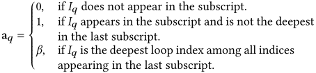
Definition 1 (Reference Access Vector) Consider a nested loop structure with n loop indices (I₁, I₂, …, I_n) and an array reference A[s₁, s₂, …, s_m] with m subscripts. We define the reference access vector for this reference as

For each q ∈ {1, …, n}, the remaining entries are defined as follows:

■

Unlike a classical dependence direction vector θ ∈ { <, =, > }ⁿ, which relates the source and sink iterations of a dependence at each loop level [3], SALT's access vector a ∈ {0, 1, β}^{n + 1} describes a single array reference: each component after the leading zero records whether a loop index is absent, present, or selected to model spatial reuse.

The synthetic leading zero is an outer position that models two consecutive executions, allowing a first-touch access to receive a finite inter-run reuse interval (inter-run RI) from the last access to the same location in the preceding execution. The usual reuse-indicator calculation handles the leading zero and any zero entries that follow it, so the inter-run RI is the first RI class encountered from outermost to innermost. When modeling one finite execution, Section 3.2 treats the corresponding first accesses as compulsory misses.

When spatial reuse is not considered, the β marker is treated as equivalent to 1, and the access vector reduces to a standard binary vector representing temporal reuse only. If multiple loop indices appear in the last subscript, the innermost loop index is marked with β, while the others are marked with 1.

Conceptually, the access vector bridges syntax and locality. Entries equal to 1 or β identify loops that move the reference to a new element or block, while entries equal to 0 identify loops across which the same element or block may later be revisited. Thus the vector is not just a compact encoding of the subscript expression; it determines which loop boundaries can contribute reuse intervals.

Example. Consider a loop nest over (i, j, k, l, m) and the following references:

A[m, i]: The last subscript is i, so the access vector is:
B[k, j + i]: The innermost loop index is j among the last subscripts (j + i), so the access vector is:

Definition 2 (Reuse Interval Position Identification)

Let a = [a₀, a₁, …, a_n] ∈ {0, 1, β}^{n + 1}, with a₀ = 0, be the access vector of a reference. The Zero Count at position i ∈ {0, …, n} is defined as the number of 0s to the right of i:

where 1_{{ · }} is the indicator function.

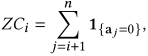
A distinct reuse interval value arises at vector position i when the Reuse Indicator χ_{RI, i} is 1. This happens when the zero count at i is stable, marking the point where all deeper loops have finished contributing to the reuse pattern and position i triggers the reuse interval occurrence. Formally, we define the Reuse Indicator Vector χ_RI ∈ {0, 1}^{n + 1} as:

Here, ZC_{− 1} ≠ ZC₀ and ZC_{n + 1} = ZC_n = 0 are boundary conventions, and a_{n + 1} is out of bounds. This indicator identifies the positions in the loop nest where we can derive a reuse interval value.

■

Example. Consider a loop nest over (i, j, k, l, m) and the reference A[i, l]. The access vector is: $𝐚 = [0100 𝛽 0]$

The computed zero counts and reuse indicators are:

Vector Position	$0$	1	2	3	4	5
Access Vector (a)	$0$	1	0	0	β	0
Zero Count (ZC)	3	3	2	1	1	0
Reuse Indicator (χ_RI)	1	0	0	1	0	1

The reuse interval values are thus identified at vector positions 0, 3, and 5, where χ_RI = 1.

■

Intuitively, a 0 in the access vector means that the corresponding loop does not change the referenced element or block. The Zero Count is the number of such reuse-preserving loops below a given level. When Zero Count drops and then stabilizes, the loop boundary marks the completion of one distinct reuse pattern, so a new reuse interval value is recorded there. This is why zero counts and reuse indicators matter for cache behavior: they identify exactly the loop levels that contribute mass to the reuse interval distribution.

The following derivation uses two levels of detail. Sections 2.5 and 2.6 gives an asymptotic temporal-only derivation, and Section 2.7 applies the same asymptotic formula with the spatial marker β to expose the temporal-spatial reuse classes. The cache model's exact temporal-spatial value formula appears in Section 2.7.2; it retains the symbolic contributions and cancellations introduced by the affine access function and includes the cache block correction induced by β.

2.5 Temporal Reuse Interval Values

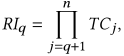
We first isolate temporal locality, where a reuse interval counts the number of accesses between two consecutive accesses to the same array element. For the running example in Section 2.3, the reference A[j][k] is independent of loop variable i and depends on loop variables j and k. According to Definition 1, its temporal-spatial access vector is $[001 𝛽],$ where β marks the innermost index contributing to spatial locality. In a temporal-only analysis, β is treated as an ordinary dependence, giving the simplified access vector $[0011] .$ By Definition 2, this vector has a single reuse-indicator position, at loop level 1. Intuitively, loop i does not change A[j][k], so the same elements are revisited across different i iterations after the inner loops over j and k complete.

Definition 3 (Asymptotic Reuse Interval Values) Given the access vector a = [a₀, a₁, …, a_n], a distinct reuse interval value can be derived at any position q ∈ {0, …, n} where χ_{RI, q} = 1. The asymptotic reuse interval value associated with this position q is:

where TC_j is the trip count of loop j and n is the total number of loops. This formula gives the reference-level RI; the kernel-level conversion follows the convention stated above.

■

For the running example, the asymptotic reuse interval value at loop level 1 is the product of the trip counts of the inner loops j and k, each with trip count n: $𝑅 𝐼 1 = \prod 3 𝑗 = 2 𝑇 𝐶 𝑗 = 𝑛 \cdot 𝑛$

This asymptotic derivation provides the value formula used later for temporal-spatial reuse. The exact temporal-spatial derivation in Section 2.7.2 keeps the lower-order and cache block correction terms omitted here.

2.6 Temporal Reuse Interval Portions

In the asymptotic temporal-only derivation, the portion of each reuse interval is calculated as:

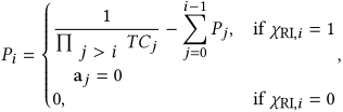
where P_i denotes the portion of the reuse interval at vector position i, and TC_j is the trip count of loop j. By convention, a product over an empty set (when no loop j > i has a_j = 0) is defined as 1.

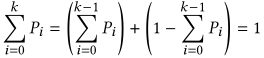
For the running example in Section 2.3, the only temporal reuse interval value is derived at loop level 1. In the simplified access vector $[0011]$ , there are no deeper zero entries after level 1, so the product in the denominator is empty and equals 1. Since no earlier nonzero portion has been assigned, the entire temporal distribution mass belongs to this interval: P₁ = 1.

Proof of Total Portion Equaling One. We verify that the sum of all reuse interval portions equals 1. Let P_i denote the portion associated with the reuse interval RI_i, and assume the final reuse interval's portion is: $𝑃 𝑘 = 1 - \sum 𝑘 - 1 𝑖 = 0 𝑃 𝑖$ .

By construction, each P_i subtracts the sum of prior portions from the cumulative fraction of total execution instances contributing to the i-th interval. Since the final interval accounts for the remainder, it completes the distribution:

■

2.7 Temporal-Spatial Reuse Interval Values

2.7.1 Asymptotic Temporal-Spatial Reuse Interval Values. We now re-derive reuse intervals while accounting for spatial locality. A temporal-spatial reuse interval is the number of accesses between consecutive accesses to the same cache block, where each block contains b array elements. Under row-major layout, spatial reuse occurs when consecutive elements in the last (rightmost) array dimension are accessed with unit stride. We assume each array dimension is larger than a cache block and that contiguous dimensions are aligned to b-element block boundaries.

To integrate spatial locality, we represent the last subscript of an array reference symbolically as β in the access vector (see Definition 1). For example, consider array reference A[k, i, m] within a 5-dimensional loop nest indexed by i, j, k, l, m, each looping n times. The access vector for reference A[k, i, m] is: $[01010 𝛽]$ , and its zero counts and reuse indicators are computed as follows:

Vector Position	$0$	1	2	3	4	5
Access Vector (a)	$0$	1	0	1	0	β
Zero Count (ZC)	2	2	1	1	0	0
Reuse Indicator (χ_RI)	1	0	1	0	1	1

Eventually, we have four distinct reuse interval values at vector positions 0, 2, 4, and 5 where χ_RI = 1, yielding: n⁵, n³, n¹, and n⁰ = 1 correspondingly using Definition 3 as the asymptotic value formula.

2.7.2 Exact Temporal-Spatial Reuse Interval Values. The asymptotic temporal-spatial analysis exposes the dominant reuse structure, but it suppresses lower-order corrections from the affine subscripts and cache block reuse. Exact temporal-spatial reuse intervals must account for whether each loop index appears in the reference subscripts and for the block size correction induced by the spatial marker β. This subsection keeps these symbolic contributions explicit and derives the reuse-interval values used by the cache model.

We first assign each vector position l ∈ {0, …, n} a reuse factor, which measures the iteration count contributed by the loops nested inside that position. The reuse factor RF_l is the product of the trip counts of all deeper loops:

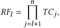
where n is the total number of loops in the nest and TC_j is the trip count of the jth loop. If there are no positions j > l, the product is over an empty set and is defined to be 1.

Whether a reuse factor increases or decreases the exact temporal-spatial reuse interval depends on the corresponding access-vector entries. The reuse interval at vector position l is computed as follows:

Add RF_j for each j > l such that χ_{RI, j} = 1 and either χ_{RI, j + 1} = 0 or a_j = β.
Subtract RF_j for each j > l such that χ_{RI, j} = 0 and χ_{RI, j + 1} = 1, treating out-of-bounds χ_{RI, j + 1} as 0.
If the access vector contains a spatial marker β at a deeper position s, subtract b · RF_s when l < s, where b is the cache block size in elements.

Putting it all together, the exact temporal-spatial reuse interval value at vector position l, denoted RI_l, is computed as:

2.8 Temporal-Spatial Reuse Interval Portions

We now extend the portion calculation to incorporate both temporal and spatial reuse. Let the access vector be $𝐚 = [𝑎 0, 𝑎 1, \dots, 𝑎 𝑛] \in {0, 1, 𝛽} 𝑛 + 1, 𝑎 0 = 0,$ under a row-major layout. Let b denote the cache block size (in elements).

Temporal Reuse Portion. For any vector position i where χ_{RI, i} = 1 and no spatial marker β appears in a before or at i, the reuse interval portion P_i is computed as in the purely temporal case:

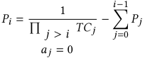
These portions reflect the share of reuse-interval occurrences attributable to temporal reuse at each index before spatial redistribution.

Spatial Reuse Adjustment. When a spatial marker β appears in the access vector at index s, we adjust earlier temporal portions as follows:

For each temporal portion P_i where i < s, divide the portion by the cache block size b.
The total reduced portion (i.e., the sum of all reductions from i < s) is reallocated to the nearest subsequent index j ≥ s where χ_{RI, j} = 1.

This redistribution scales earlier temporal portions to account for intra-block reuse and assigns the removed mass to the next block-level reuse point.

2.9 Worked Examples

This section illustrates SALT on two cases: single-level tiled matrix multiplication and a 5-point stencil. The same matrix-multiplication procedure applies to deeper tiling; we omit the full two-level derivation and report only its final result in Section 3.2.

2.9.1 Tiled Matrix Multiplication. We use single-level tiled matrix multiplication as the worked example. Given tile dimensions t_m and t_n, matrices may be divided into sub-blocks as follows:

The corresponding tiled loop nest is:

for (int i = 0; i < n; i += t_m)
  for (int j = 0; j < n; j += t_n)
    for (int k = 0; k < n; k += t_m)
      for (int ii = 0; ii < t_m; ii++)
        for (int jj = 0; jj < t_n; jj++)
          for (int kk = 0; kk < t_m; kk++)
            C[i+ii][j+jj] += A[i+ii][k+kk]
                             * B[k+kk][j+jj];

We now apply the exact temporal-spatial computation from section 2.7.2 to the reference B[k + kk][j + jj] in tiled matrix multiplication. For this reference, the access vector is $[00110 𝛽 1],$ so Definition 2 identifies reuse levels i, ii, and jj (levels 1, 4, and 5), where χ_RI = 1. The reuse factors derived from the loop trip counts are:

Level	Indices	TC	χ_RI	Reuse Factor
0	N/A	N/A	0	n³
1	i	n/t_m	1	$𝑛 𝑡 𝑛 \times 𝑛 𝑡 𝑚 \times 𝑡 𝑚 \times 𝑡 𝑛 \times 𝑡 𝑚 = 𝑛 2 \times 𝑡 𝑚$
2	j	n/t_n	0	$𝑛 𝑡 𝑚 \times 𝑡 𝑚 \times 𝑡 𝑛 \times 𝑡 𝑚 = 𝑛 \times 𝑡 𝑚 \times 𝑡 𝑛$
3	k	n/t_m	0	$𝑡 𝑚 \times 𝑡 𝑛 \times 𝑡 𝑚 = 𝑡 2 𝑚 \times 𝑡 𝑛$
4	ii	t_m	1	t_n × t_m
5	jj	t_n	1	t_m
6	kk	t_m	0	1

Applying the same construction at the reuse levels jj, ii, and i, where χ_RI = 1, gives the complete reuse interval distribution for reference B:

No.	Level	ri construction for reference B	P_ri
1	jj	RF₅ = t_m	$1 - 1 𝑏$
2	ii	RF₄ + RF₅ − b · RF₅ = t_m · t_n + t_m − b · t_m	$1 𝑏 - 1 𝑏 \cdot 𝑡 𝑚$
3	i	RF₁ + RF₄ + RF₅ − RF₃ − b · RF₅ = n² · t_m + t_m · t_n + t_m $- 𝑡 2 𝑚 \cdot 𝑡 𝑛 - 𝑏 \cdot 𝑡 𝑚$	$1 𝑏 \cdot 𝑡 𝑚$

Following the reuse interval and reuse distance analysis conventions for matrix multiplication established by Smith et al. [35], we adopt a 3-access model, reflecting the three array references in the innermost loop. Under the kernel-level conversion above, the reuse interval values for reference B are multiplied by 3 and the corresponding portions are divided by 3.

2.9.2 Constant-Offset Group Reuse for Stencils. For stencil-style group reuse, SALT first derives the ordinary reference-level RI distribution after ignoring constant shifts, then uses the fixed chronological dynamic order of the shifted references to intercept long self-reuse intervals. Consider the interior points of the 5-point stencil:

Boundary and block-divisibility effects are outside this interior-pattern derivation. After constant offsets are ignored, all five references to A share the same access vector

[01 𝛽],

where β marks the innermost loop index that contributes cache block spatial reuse; under row-major layout, the output reference B[i][j] has the same access vector. Before the group reuse adjustment, SALT therefore assigns each A reference and the B reference the same reference-level distribution:

where TC_i and TC_j are the trip counts of the outer and inner stencil loops and b is the number of array elements per cache block.

For a fixed element A[x][y], a shifted reference A[i + δ_i][j + δ_j] touches that element at loop instance (i, j) = (x − δ_i, y − δ_j). With i outer and j inner, the chronological dynamic order of the five shifted references is

and the body-instance displacements between adjacent touches are

These displacements count loop-body executions between two shifted references touching the same A element. Thus, group reuse replaces the long interval TC_iTC_j + 1 − b for four of the five shifted A references: two references become P(ri = 1) = 1, two become

𝑃 (r i = 1) = 1 - 1 𝑏

and

𝑃 (r i = 𝑇 𝐶 𝑗 - 1) = 1 𝑏

, and one keeps

𝑃 (r i = 1) = 1 - 1 𝑏

and

𝑃 (r i = 𝑇 𝐶 𝑖 𝑇 𝐶 𝑗 + 1 - 𝑏) = 1 𝑏

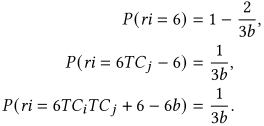
The loop body has six static memory references: five loads from A and one access to B. Following the same convention used above, each reference-level RI value is multiplied by 6 and each reference-level portion is divided by 6. Combining the five A distributions with the unchanged B distribution gives the kernel-level RI distribution:

The three probabilities sum to 1. This distribution is then passed to Denning's recursion in the same way as the other SALT-derived RI distributions to obtain the miss-ratio curve.

3 From Reuse-Interval Distributions to Miss-Ratio Curves

The preceding analysis produces symbolic RI values and their portions. This section uses Denning's working-set theory [10] to convert SALT's symbolic RI distribution into an approximate miss-ratio curve.

3.1 Working-Set Model

At any point in an access trace, the working set for a window of length x is the set of distinct data blocks accessed by the most recent x references. A working-set cache retains exactly these blocks. Logical time advances once per memory reference, so x is measured in references rather than wall-clock time. Working sets were originally developed for virtual-memory management [11, 12]; here, we use the number of blocks in the working set as a cache-capacity estimate.

Let P(ri = v) be the portion of accesses having reuse interval v; together, these portions form the RI distribution. An access misses for window length x if and only if ri > x. Denning's recursion [12] therefore gives the time-window miss ratio m(x) and the expected number of distinct blocks in the window, s(x):

𝑚 (𝑥) = 𝑃 (r i > 𝑥), 𝑠 (0) = 0, 𝑠 (𝑥 + 1) = 𝑠 (𝑥) + 𝑚 (𝑥) .

(1)

The recursion starts with an empty window. Extending it from x to x + 1 adds a distinct block exactly when the newly included reference has ri > x, an event with probability m(x). Repeated application gives

𝑠 (𝑥) = \sum 𝑥 - 1 𝑦 = 0 𝑚 (𝑦)

A working-set cache fixes x, whereas an LRU cache fixes its capacity. Denning connects them by setting the LRU capacity to the expected working-set size [12]:

𝑐 (𝑥) = 𝑠 (𝑥) = 𝑥 - 1 \sum 𝑦 = 0 𝑚 (𝑦), m r (𝑐 (𝑥)) \approx 𝑚 (𝑥) .

(2)

This LRU approximation maps x to capacity c(x) and miss ratio m(x). Since s(x) is an expectation, c(x) may be fractional. For an integer capacity between two such points, the neighboring m(x) values bound the miss ratio by monotonicity.

3.1.1 Constructing the Miss-Ratio Curve. SALT takes the symbolic RI values and portions produced by the preceding analysis as input. Only RI values with nonzero portions affect m(x); SALT therefore visits those values instead of enumerating every logical time x. Let the distinct positive RI values, augmented with an initial zero, be

where p₀ = 0 and

\sum 𝑘 𝑖 = 1 𝑝 𝑖 = 1

. Before accounting for first accesses in a finite execution, the miss ratio at ri_i is the RI tail:

𝑚 (r i 𝑖) = 𝑘 \sum 𝑗 = 𝑖 + 1 𝑝 𝑗 (0 \leq 𝑖 < 𝑘), 𝑚 (r i 𝑘) = 0 .

(3)

Because there is no RI mass between ri_i and ri_{i + 1}, m(x) is constant at m(ri_i) throughout this interval. Applying Equation (1) over the ri_{i + 1} − ri_i unit steps gives

𝑐 (r i 0) = 0, 𝑐 (r i 𝑖 + 1) = 𝑐 (r i 𝑖) + 𝑚 (r i 𝑖) (r i 𝑖 + 1 - r i 𝑖) .

(4)

where c(ri₀) = c(0) = 0. Unrolling the recurrence gives

𝑐 (r i 𝑖) = 𝑖 - 1 \sum 𝛾 = 0 𝑚 (r i 𝛾) (r i 𝛾 + 1 - r i 𝛾) .

(5)

Each breakpoint yields a preliminary LRU pair (c(ri_i), m(ri_i)). SALT performs one symbolic update per gap, or k updates independent of the RI magnitudes. It applies the compulsory-miss correction below only after completing this sparse calculation.

3.2 Parametric Miss-Ratio Curves

3.2.1 Compulsory-Miss Correction. The leading-zero construction treats the analyzed execution as following an identical preceding execution. It therefore assigns each first access to a block a finite inter-run RI, measured from the block's last access in the preceding execution. For a static reference r, let q be the first access-vector position, from the synthetic leading zero toward the innermost loop, for which $𝜒 (𝑟) R I, 𝑞 = 1$ . Let $𝑅 𝐼 (𝑟) 𝑞$ be the corresponding reference-level RI. Because the full kernel trace contains R memory references per loop-body execution, the kernel-level inter-run RI is

𝐻 (𝑟) = 𝑅 \cdot 𝑅 𝐼 (𝑟) 𝑞 .

(6)

When modeling a single execution, the preceding access does not exist. These first accesses are therefore compulsory misses at every cache capacity. Let $𝐚 (𝑟) = [0, 𝑎 (𝑟) 1, \dots, 𝑎 (𝑟) 𝑛]$ be the access vector of r. Their portion of the total accesses in that execution is

𝜅 (𝑟) = 1 𝑅 𝑏 \prod 1 \leq 𝑗 \leq 𝑛 𝑎 (𝑟) 𝑗 = 0 𝑇 𝐶 𝑗 .

(7)

The portion computed in Section 2.8 for this outermost RI class can mix first accesses with accesses that are reused within the same execution. To extract only the compulsory portion, the product above includes every zero component: each such loop repeats the same address sequence and contributes a factor 1/TC_j. The additional factor 1/b converts element accesses to first accesses per block, while 1/R normalizes across the R static references. Thus κ^(r) is the first-access component, rather than the entire portion, of the outermost RI class.

SALT first completes the sparse cache-size calculation in Equations (3) and (5). It then revisits the resulting miss-ratio points. For every pair (H^(r), κ^(r)), SALT adds κ^(r) to each point whose RI is at least H^(r):

𝑚 (r i 𝑖) \leftarrow 𝑚 (r i 𝑖) + \sum 𝑟 : 𝐻 (𝑟) \leq r i 𝑖 𝜅 (𝑟) .

(8)

This second pass updates the miss ratios at the previously computed cache sizes. At the largest breakpoint, every correction applies, so the curve ends at the compulsory miss ratio m(ri_k) = ∑_rκ^(r) rather than zero.

Table 5: Cache size and miss ratio for two untiled loop orders.

Loop Order	IJK		IKJ
ri_i	c(ri_i)	m(ri_i)	c(ri_i)	m(ri_i)
0	0	1	0	1
3	3	$13 + 1 3 𝑏 + 1 3 𝑏 𝑛$	3	$2 3 𝑏 + 1 3 𝑏 𝑛$
3n	$𝑛 + 𝑛 𝑏$	$1 3 𝑏 + 2 3 𝑏 𝑛$	$2 𝑛 𝑏$	$1 3 𝑏 + 2 3 𝑏 𝑛$
3n²	$𝑛 2 𝑏$	$1 𝑏 𝑛$	$𝑛 2 𝑏$	$1 𝑏 𝑛$
3n³	$3 𝑛 2 𝑏$	$1 𝑏 𝑛$	$3 𝑛 2 𝑏$	$1 𝑏 𝑛$

For example, consider the dominant-term summary of three-access IJK matrix multiplication in Table 1. Each of A[i, k], B[k, j], and C[i, j] has compulsory portion 1/(3bn). Their kernel-level inter-run RIs are H^(B) = 3n² and H^(A) = H^(C) = 3n³. Before correction, the sparse calculation gives m(3n²) = 2/(3bn) and m(3n³) = 0. The second pass produces

The corrected values are equal, so 3n³ is no longer a turning point, but Table 1 retains it to show the correction. Where shown, P(ri) and c(ri) come from the initial sparse calculation, while m(ri) includes the second-pass correction.

Table 6: Parametric RI distribution, cache size, and miss ratio for single-level tiled matrix multiplication.

ri_i	P(ri_i)	c(ri_i)	m(ri_i)
0	0	0	1
3	$2 𝑏 𝑡 𝑚 - 𝑡 𝑚 - 1 3 𝑏 𝑡 𝑚$	3	$13 + 1 3 𝑏 + 1 3 𝑏 𝑡 𝑚$
3t_m	$𝑏 𝑡 𝑛 - 1 3 𝑏 𝑡 𝑛$	$𝑡 𝑚 + 𝑡 𝑚 𝑏$	$1 3 𝑏 + 1 3 𝑏 𝑡 𝑚 + 1 3 𝑏 𝑡 𝑛$
3t_mt_n	$𝑡 𝑚 - 1 3 𝑏 𝑡 𝑚$	$𝑡 𝑚 + 𝑡 𝑚 𝑡 𝑛 𝑏$	$2 3 𝑏 𝑡 𝑚 + 1 3 𝑏 𝑡 𝑛$
$3 𝑡 2 𝑚 𝑡 𝑛$	$𝑛 - 𝑡 𝑛 3 𝑏 𝑛 𝑡 𝑚$	$𝑡 𝑚 + 𝑡 2 𝑚 + 3 𝑡 𝑚 𝑡 𝑛 𝑏$	$1 3 𝑏 𝑡 𝑚 + 1 3 𝑏 𝑡 𝑛 + 1 3 𝑏 𝑛$
3nt_mt_n	$𝑛 - 𝑡 𝑛 3 𝑏 𝑛 𝑡 𝑛$	$3 𝑡 𝑚 𝑡 𝑛 + 𝑡 𝑚 𝑛 + 𝑡 𝑛 𝑛 𝑏$	$1 3 𝑏 𝑡 𝑚 + 2 3 𝑏 𝑛$
3n²t_m	$1 3 𝑏 𝑛 𝑡 𝑚$	$𝑡 𝑚 𝑡 𝑛 + 3 𝑡 𝑚 𝑛 + 𝑛 2 𝑏$	$1 𝑛 𝑏$

SALT can analyze a loop nest in any loop order. Table 1 compares two common untiled orders, IJK and IKJ, for square n × n matrices. Table 2 gives the closed-form RI distribution, cache size, and miss ratio for single-level tiled matrix multiplication with rectangular tiles of size t_m × t_n. These expressions remain symbolic in the problem size, tile dimensions, and cache block size, so changing a tile configuration does not require rerunning the analysis. The same procedure extends to deeper tiling; Section 5.2 and Table 3 evaluate both single- and two-level tiled kernels.

SALT computes reuse interval values and portions as parametric polynomial expressions that capture both temporal and spatial reuse. These closed forms expose how the problem size n, tile sizes t_m and t_n, and cache block size b affect the miss ratio across a large configuration space.

4 Compiler Implementation

4.1 MLIR Input Representation

The implementation accepts kernels represented in an MLIR-based toolchain [26]. A kernel may contain one or more regular rectangular loop nests. Each loop bound is a symbolic expression in values defined outside the containing loop nest and is independent of surrounding loop indices, while array subscripts are affine in the loop indices. The whole kernel need not be one perfectly nested loop. Our implementation converts the MLIR input program into an inductively defined tree structure and analyzes each memory reference with respect to the loop nest that syntactically contains it. We treat any SSA values defined outside the containing loop nest as symbolic parameters.

4.2 Analyzer Implementation

SALT analyzes the loop tree recursively, moving from outer loops toward individual memory references. During this traversal, the analyzer maintains two symbolic quantities: reuse factors, which count how often each reuse class occurs, and trip counts, which describe the iteration space at each loop level. The reuse-interval distribution is derived from these quantities.

For each memory reference, SALT constructs an access vector that records how the array subscripts depend on the loop induction variables. The access vector determines which loop levels can generate temporal reuse and which level can generate cache block reuse. To model spatial locality, SALT introduces a symbolic cache block size b and uses it to distinguish intra-block reuse from inter-block reuse. Keeping b symbolic lets the analysis produce miss-ratio expressions parameterized by cache block size even when b occurs as a divisor, a form that standard Presburger arithmetic cannot directly encode.

We implement SALT in Rust [24]. The implementation uses Rust's type system and ownership model to keep the recursive analysis explicit and memory safe, and it relies on Symbolica [34] for symbolic arithmetic over rational polynomials.

5 Evaluation

We evaluate SALT along three dimensions: analysis cost, agreement with cache simulation, and agreement with hardware counters. We compare against Cachegrind simulation and a polyhedral counting baseline implemented using Barvinok. The experiments use two workload groups: matrix multiplication under increasing tiling depth, and a suite of affine tensor kernels generated through an MLIR tiling pipeline.

5.1 Experimental Methodology

5.1.1 Cache-Simulation Baseline. Cachegrind [29] observes the dynamic memory-access trace, simulates cache behavior, and reports miss counts. It requires a fully instantiated program and scales with dynamic execution length, so its results are numerical rather than symbolic.

5.1.2 Polyhedral Counting Baseline. Previous techniques [4, 5, 39] use the polyhedral model to represent iteration domains, memory accesses, and reuse relations with affine constraints, then count integer points in the resulting parametric polyhedra. We implement this comparison using the Barvinok library [38]. For each access, the baseline relates it to its lexicographically latest preceding access to the same location and counts the distinct memory locations accessed in between. This formulation supports a broader class of affine programs than SALT, including affine conditionals and index-dependent bounds. However, standard Presburger/polyhedral formulations cannot directly encode tile or cache-block sizes when those parameters remain symbolic and occur as variable strides, coefficients, or divisors. The reported timings characterize this Barvinok-based implementation rather than all polyhedral analyses.

5.1.3 Workloads and Platforms. We evaluate two workload groups: matrix multiplication under untiled, single-level tiled, and two-level tiled configurations, and a suite of eight affine tensor kernels covering tensor contractions, attention primitives, BLAS-like kernels, and rowwise softmax. Matrix-multiplication experiments run on an AMD Ryzen 9950X with 16 cores and 32 threads; tensor-kernel experiments run on an Intel Core i7–7700 with 4 cores and 8 threads. We execute independent Cachegrind configurations concurrently, using at most one Cachegrind process per hardware thread; all reported analysis times are end-to-end wall-clock times. These experiments evaluate the accuracy and efficiency of SALT's locality analysis, not the runtime performance of the analyzed kernels.

5.1.4 Data Layout. We pad arrays to reduce conflict misses and to match common layout optimizations. The innermost, contiguous dimension is rounded to 8p, where 8 is the cache block size in elements and p is the smallest prime such that 8p ≥ d_original. Intermediate dimensions are rounded up to the nearest prime. The outermost dimension is left unchanged. This configuration is intended to reduce conflict misses. For a general approach under different tile configurations and compiler optimizations (such as vectorization and unrolling), one must consider the tile footprint and cache mapping together [19].

5.1.5 Cache-Simulation Configuration. Each benchmark is compiled as a minimal executable whose dynamic trace consists only of the measured loop nest. The kernel is placed at the _start entry point, compiler memory fences prevent load/store elimination or reordering, and the program exits immediately after the loop nest.

We invoke Cachegrind with explicit L1 data-cache configurations. Fully associative experiments use 64-byte blocks, and timing experiments sweep capacities from 2 to 1024 blocks unless otherwise stated. Set-associative experiments use 64-byte lines, associativity A ∈ {8, 12}, and 2ⁱ sets, for total capacity 64 × A × 2ⁱ bytes, where 2 ≤ 2ⁱ ≤ 128. We choose 8-way and 12-way associativity to reflect common L1 data-cache configurations.

5.2 Matrix Multiplication

5.2.1 Analysis Cost. Table 3 compares SALT with the polyhedral counting baseline under symbolic and concrete problem dimensions and with Cachegrind simulation. We evaluate these approaches on three matrix-multiplication kernels: no tiling, single-level tiling, and two-level tiling. Parameter treatment differs across the three methods. SALT keeps the problem dimensions, tile sizes, and cache block size symbolic. The symbolic-input Barvinok baseline keeps only the problem dimensions symbolic; it fixes the cache block size to b = 8, the single-level tile size to 32 × 32, and the two-level tile sizes to 128 × 128 and 32 × 32. The concrete-input Barvinok and Cachegrind experiments additionally set M = N = K to either 256 or 512.

Table 7: Analysis and simulation time (seconds) for matrix multiplication under different tiling levels.

Method	Configuration	No Tiling	1-Level	2-Level
SALT	Symbolic input,symbolic tiles	0.007	0.007	0.007
Barvinok	Symbolic input,block size 8, tiles 32/128	0.17	3.75	89.2
Barvinok	Input size 256	0.13	1.41	24.3
Barvinok	Input size 512	0.12	1.40	31.3
Simulation	Input 256, tiles 32/128	220	57.9	59.2
Simulation	Input 512, tiles 32/128	2789	474	445

As Table 3 shows, SALT takes about 7 ms on each kernel because it is fully parametric in input dimensions, tile sizes, and cache parameters. The Barvinok-based polyhedral baseline grows rapidly with tiling depth: with symbolic input dimensions, it rises from 0.17 s on the untiled kernel to 89.2 s on the two-level tiled kernel, and the concrete-input cases show the same trend. Simulation is much slower and scales with dynamic work: for n = 512, the untiled kernel takes 2789 seconds, and the two-level tiled kernel still takes 445 seconds, even when running the cache simulations in parallel across all hardware threads. For two-level tiled matrix multiplication, SALT is approximately 12, 700 × faster than the symbolic polyhedral baseline; across the evaluated matrix-multiplication configurations, its speedup over simulation ranges from approximately 8, 300 × to 398, 000 ×. To keep the timing study manageable, these simulations sweep capacities only up to 1024 blocks.

Figure 1: Matrix-multiplication miss ratios predicted by SALT (dashed lines) and simulated by Cachegrind (markers) for n = 256: untiled, one-level tiled with 32 × 32 tiles (T1), and two-level tiled with 128 × 128 outer and 32 × 32 inner tiles (T2). Cache capacity is measured in 64-byte blocks (b = 8 array elements).

We compare SALT's predictions against Cachegrind for n = 256 under three tiling configurations: untiled, single-level tiled with 32 × 32 tiles (T1), and two-level tiled with 128 × 128 outer tiles and 32 × 32 inner tiles (T2). All runs use a fully associative LRU cache with a block size b = 8 elements (64 bytes per block).

5.2.2 Prediction Accuracy. Figure 1 plots miss-ratio curves over a broad range of cache capacities, with Cachegrind validation at selected capacities throughout the plotted range. Across all three kernels, SALT reconstructs the plateau levels and sharp drops at the cache-capacity thresholds derived from the reuse-interval distribution. The mean absolute percentage error remains under $15 %$ , and the mean squared error is below 6.4 × 10^{− 4} in every configuration, so both the level and shape of the miss-ratio curves are captured. This MAPE is computed across cache capacities for the matrix-multiplication curves; it is therefore not directly comparable with the hardware MAPE in Figure 4, which is computed across kernels at one physical cache configuration.

The untiled kernel shows a single prominent drop: once the cache can hold a full row of A and a column of B, the miss ratio drops sharply. Tiling introduces additional reuse scales and, therefore, more turning points: it adds a drop when a 32 × 32 tile fits in the cache.

The large-cache region on the right side of Figure 1 exposes a nonmonotone difference between T1 and T2. For small and medium cache sizes, their miss ratios are similar and both improve substantially over the untiled kernel. T2 has fewer misses over much of the large-cache region, but T1 reaches its compulsory-miss floor first, near 10⁴ blocks. T2 therefore has a slightly higher miss ratio until its next drop, near 2 × 10⁴ blocks, after which the two configurations converge.

In SALT's model, the extra outer tiling level introduces long inter-tile reuse intervals and hence an additional capacity threshold; it does not inherently improve spatial locality, because T1 and T2 use the same 32 × 32 inner tile and cache block size. More generally, effective tile sizes depend on cache capacity, cache organization, and data layout, and multilevel tile selection is therefore an optimization problem rather than a guarantee of monotonic improvement [9, 25, 27]. SALT exposes this configuration-specific behavior through the additional turning points in the T2 reuse-interval distribution.

5.3 Tensor Kernel Suite

SALT analyzes a suite of affine tensor kernels through its MLIR-based compiler flow. The suite includes 3D tensor-vector contraction, 4D tensor contraction, attention context lookup, attention score, batched GEMM, matrix-matrix contraction, matrix-vector contraction, and rowwise softmax. Rowwise softmax includes non-affine arithmetic, but its loop bounds and memory accesses are affine; SALT analyzes this cache-relevant access structure. We evaluate both original and tiled versions of each kernel.

We generate tiled variants with MLIR tiling, normalization, and canonicalization passes: we use a tile size of 8, remove single-iteration levels, and simplify affine expressions.

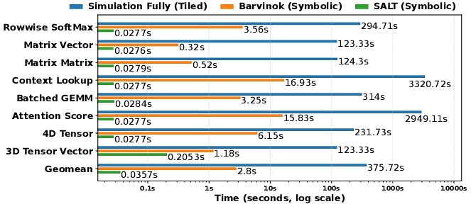
Figure 2: End-to-end evaluation time on an Intel Core i7–7700 for the tiled tensor kernels using fully associative Cachegrind simulation, the Barvinok-based polyhedral counting baseline, and SALT. Times are in seconds on a logarithmic scale; the geometric mean is taken across the eight kernels.

5.3.1 Analysis Cost. SALT's symbolic evaluation eliminates runtime enumeration of reuse intervals and cache states, so its analysis time does not scale with concrete data sizes or tile extents; it still depends on static program structure and symbolic-expression complexity. Figure 2 reports per-kernel evaluation times for tiled kernels across fully associative simulation, the Barvinok-based polyhedral baseline, and SALT. The geometric-mean times are 0.0357 seconds for SALT, 2.80 seconds for the polyhedral baseline, and 375.72 seconds for simulation. SALT is therefore approximately 78 × faster than the polyhedral baseline and 11, 000 × faster than simulation.

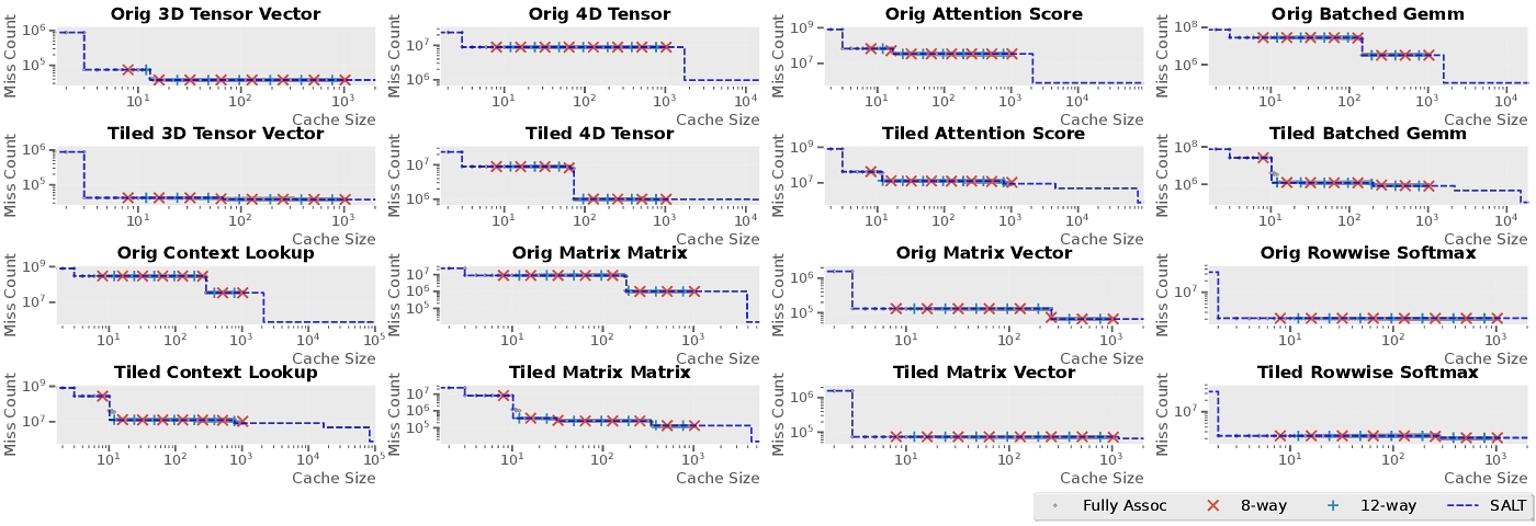
Figure 3: Miss counts predicted by SALT (dashed lines) and obtained by fully associative, 8-way, and 12-way cache simulation for the original and tiled variants of eight tensor kernels. Cache capacity is measured in 64-byte blocks; simulation points extend through 1,024 blocks.

5.3.2 Simulation Accuracy. Figure 3 compares SALT predictions with fully associative, 8-way, and 12-way cache simulations. The 8-way and 12-way simulations test how closely the fully associative LRU baseline tracks set-associative caches for the padded layouts used in our experiments. The simulations sweep L1D capacities up to 1,024 blocks, corresponding to 64 KiB with 64-byte cache blocks. Across the evaluated kernels, the simulated curves closely track SALT's analytical prediction: the plateaus and drops appear at the cache-capacity thresholds derived from the reuse-interval distributions for both untiled and tiled variants.

Tiling reduces the effective footprint of reuse clusters, shifting drops to smaller cache sizes and lowering plateau heights in kernels such as tiled-batched-gemm, tiled-context-lookup, and tiled-matrix-matrix. For the evaluated kernels and padded layouts, the 8-way and 12-way results closely track the fully associative baseline. This agreement does not imply that padding generally eliminates conflict misses, as aggressive tiling, vectorization, packing, or different alignments may produce substantially different set mappings. For rowwise-softmax, the miss curve becomes flat once the cache can hold several blocks of elements; both SALT and simulation then predict only the residual compulsory misses.

Overall, the symbolic analysis predicts not only aggregate miss ratios but also the piecewise structure of the miss-count curve: plateau magnitudes, turning points, and capacity transitions across tiling levels.

5.3.3 Hardware-Counter Validation. We further compare SALT predictions with measurements from processor performance monitoring counters (PMCs) on an Intel i7–7700 (Kaby Lake, 8-way, 32 KiB L1D). Each kernel was compiled with -O3 and executed on an isolated, affinity-pinned core; we collected the L1D_LOAD_MISSES event without multiplexing or scaling, with prefetchers enabled. The native kernels retain their stores but update outputs using read-modify-write accesses. When an output cache block (hardware cache line) is absent from L1D, the output load brings the block into L1D and the immediately following store hits it; the load thus captures the block fill associated with the output-store address stream modeled by SALT, without counting the subsequent store as a separate miss.

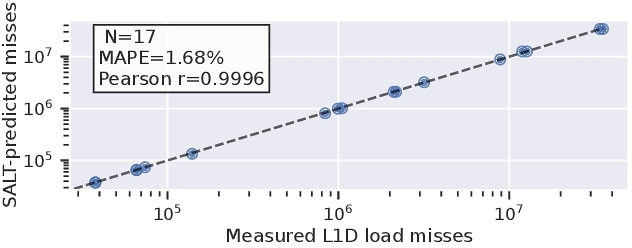
Figure 4: SALT-predicted cache misses versus L1D load misses measured on an Intel i7–7700 using a processor performance monitoring counter (PMC) event. Each point represents one hardware-validation experiment; the dashed line indicates perfect agreement (y = x).

Figure 4 shows close agreement across roughly three orders of magnitude, with mean absolute percentage error (MAPE) of $1.68 %$ and Pearson correlation r = 0.9996. The 17 validation points include the original and tiled versions of the eight tensor kernels and one untiled 512 × 512 5-point spatial stencil, analyzed using the restricted group-reuse treatment in Section 2.9.2. Because we did not disable prefetching, Figure 4 validates aggregate L1D miss prediction under the measured configuration, not prefetch behavior. SALT does not model prefetch timeliness, cache pollution, or non-LRU replacement. The signed miss-ratio errors remain within ± 0.25 percentage points and may reflect these effects, finite associativity, compiler code generation, and counter behavior.

6 Related Work

Loop tiling transforms a d-dimensional nested loop into a (k + 1)d-dimensional nested loop with k levels of tiling [42, 43]. The correctness is ensured when using rectangular tiling for fully permutable loops [41]. Many techniques choose tile shapes and sizes using heuristics [40] or optimization [43]; these classical approaches do not generally derive a complete miss-ratio curve parameterized by cache capacity, block size, and LRU replacement.

Li et al. [27] present a solver-driven model for multilevel tile size and loop permutation optimization in dense tensor contractions. Their approach exploits the tensor contraction property that each tensor dimension is indexed by a distinct loop iterator, yielding zero/full inter-tile reuse with respect to a tiling loop and allowing the permutation search to be largely pruned to the choice of the innermost tiling loop at each level. The model produces conditional data movement expressions over tile sizes and cache capacities, which a constrained nonconvex solver uses to choose concrete tile sizes. Their problem is optimization, i.e., optimal tiling for a single-level cache of a given size. Our work is complementary: SALT analyzes a given loop nest to derive an approximate fully associative LRU miss-ratio curve across cache sizes as a symbolic function of loop bounds and tile dimensions.

Tiled matrix multiplication has been a fundamental part of scientific computing, implemented in the BLAS library [13] and many optimizing compilers since the 1990s [8, 42]. It is a significant application of polyhedral compilation techniques [1, 41, 44], an essential component in the domain-specific optimization system Halide [33], and increasingly optimized on GPUs [47]. Compiler analyses must balance model generality with compilation cost. Within its supported domain, SALT runs in time proportional to the product of the number of static memory references and loop indices.

Presburger arithmetic has long been used in compiler analysis, including early loop tiling for imperfectly nested loops [22]. It is used to precisely formulate and solve for the effect of caching, such as miss-ratio equations [16], reuse-distance equations [5], and polyhedral models [4, 32]. It cannot encode multiplication between variables or division by a symbolic parameter; consequently, symbolic tile or cache block sizes must be fixed when they occur as variable strides, coefficients, or divisors. General Presburger decision procedures have a doubly exponential worst-case lower bound [18]. This bound applies to the unrestricted decision problem and does not imply that every Presburger formulation or solver run will exhibit doubly exponential behavior. Our evaluation instead shows that the Barvinok-based baseline is fast on simpler cases but grows with tiling depth, whereas SALT's analysis time remains nearly constant (Table 3). Presburger-based solvers support more general affine iteration spaces, including affine conditionals and index-dependent bounds, whereas SALT targets rectangular loop nests with loop-invariant symbolic bounds; Section 2.2 provides the detailed restrictions.

SARCASM [21] models set-associative cache behavior through detailed footprints that describe the number of cache lines mapping to each set. Their work supports tiled rectangular loops. Their results indicate the bias in set assignment for tensor contractions and provide a method to account for it in the analysis. SARCASM and SALT address complementary aspects of cache analysis: SARCASM captures set conflicts, while SALT maintains problem and tile sizes symbolically in derived reuse-interval distributions and converts them to miss ratios under a fully associative LRU model. A possible extension is to combine SALT's symbolic reuse analysis with detailed address-to-set mapping.

Padding is closely related to cache mapping. Hong et al. [19] develop padding algorithms for arbitrary tile sizes in set-associative caches and extend support to nested tiles and multilevel caches. Their work shows how padding choices affect the tile footprint and its distribution across cache sets. SALT evaluates only a simple padding heuristic and does not model the set mapping itself. Besides padding, highly optimized kernels may also utilize packing [17, 46] and vectorization [6, 37]. SALT analyzes capacity locality; set-aware layout selection is a distinct but interacting problem.

7 Conclusion

This paper has presented SALT, a compiler technique for deriving reuse-interval distributions and approximate parametric cache miss ratios for symbolically bounded rectangular loop nests with affine array accesses, including untiled and multilevel-tiled kernels. SALT represents each array reference with a reference access vector, computes the modeled temporal and spatial reuse-interval distribution in closed form, and applies Denning's working-set recursion to approximate miss ratios. Its cost is polynomial in the number of loop indices and static memory references, and is independent of tensor sizes, tile sizes, cache block sizes, and cache capacity.

We integrated SALT into an MLIR-based toolchain and applied it to tiled and untiled matrix multiplication and eight tensor kernels, including attention and batched GEMM. Across the eight tensor kernels, SALT achieves geometric-mean speedups of approximately 78 × over our Barvinok-based polyhedral counting baseline and 11, 000 × over Cachegrind simulation. These results establish the efficiency and accuracy of SALT's analysis within its stated scope. Evaluating SALT within a complete autotuning workflow and on architecture-specific optimized kernels remains future work.

References

Aravind Acharya, Uday Bondhugula, and Albert Cohen. 2018. Polyhedral auto-transformation with no integer linear programming. In Proceedings of the ACM SIGPLAN Conference on Programming Language Design and Implementation, Jeffrey S. Foster and Dan Grossman (Eds.). ACM, 529–542.
Alfred V. Aho, Monica S. Lam, Ravi Sethi, and Jeffrey D. Ullman. 2006. Compilers: Principles, Techniques, and Tools (2nd ed.). Addison-Wesley.
Randy Allen and Ken Kennedy. 2001. Optimizing Compilers for Modern Architectures: A Dependence-based Approach. Morgan Kaufmann Publishers.
Wenlei Bao, Sriram Krishnamoorthy, Louis-Noël Pouchet, and P. Sadayappan. 2018. Analytical modeling of cache behavior for affine programs. Proceedings of the ACM on Programming Languages 2, POPL (2018), 32:1–32:26. https://doi.org/10.1145/3158120
Kristof Beyls and Erik H. D'Hollander. 2005. Generating cache hints for improved program efficiency. Journal of Systems Architecture 51, 4 (2005), 223–250. https://doi.org/10.1016/j.sysarc.2004.09.004
Uday Bondhugula. 2020. High Performance Code Generation in MLIR: An Early Case Study with GEMM. (2020). arxiv:2003.00532 [cs.PL] https://arxiv.org/abs/2003.00532
Uday Bondhugula, Albert Hartono, J. Ramanujam, and P. Sadayappan. 2008. A practical automatic polyhedral parallelizer and locality optimizer. In Proceedings of the ACM SIGPLAN Conference on Programming Language Design and Implementation. 101–113.
Steve Carr and Ken Kennedy. 1992. Compiler Blockability of Numerical Algorithms. In Proceedings of the International Conference for High Performance Computing, Networking, Storage and Analysis (SC), Robert Werner (Ed.). IEEE Computer Society, 114–124.
Stephanie Coleman and Kathryn S. McKinley. 1995. Tile Size Selection Using Cache Organization and Data Layout. In Proceedings of the ACM SIGPLAN Conference on Programming Language Design and Implementation. ACM, New York, NY, USA, 279–290. https://doi.org/10.1145/207110.207162
Peter J. Denning. 1980. Working sets past and present. IEEE Transactions on Software Engineering SE-6, 1 (Jan. 1980).
Peter J. Denning. 2021. Working Set Analytics. ACM Computing Survey 53, 6 (2021), 113:1–113:36. https://doi.org/10.1145/3399709
Peter J. Denning and Stuart C. Schwartz. 1972. Properties of the working set model. Commun. ACM 15, 3 (1972), 191–198. https://doi.org/10.1145/361268.361281
Jack J. Dongarra, Jeremy Du Croz, Sven Hammarling, and Iain S. Duff. 1990. A set of level 3 basic linear algebra subprograms. ACM Trans. Math. Softw. 16, 1 (1990), 18–28.
Venmugil Elango, Fabrice Rastello, Louis-Noël Pouchet, J. Ramanujam, and P. Sadayappan. 2015. On Characterizing the Data Access Complexity of Programs. In Proceedings of the ACM SIGPLAN-SIGACT Symposium on Principles of Programming Languages. 567–580. https://doi.org/10.1145/2676726.2677010
Matteo Frigo, Charles E. Leiserson, Harald Prokop, and Sridhar Ramachandran. 1999. Cache-Oblivious Algorithms. In Proceedings of the Symposium on Foundations of Computer Science. 285–298.
Somnath Ghosh, Margaret Martonosi, and Sharad Malik. 1999. Cache Miss Equations: A Compiler Framework for Analyzing and Tuning Memory Behavior. ACM Transactions on Programming Languages and Systems 21, 4 (1999), 703–746. https://doi.org/10.1145/325478.325479
Kazushige Goto and Robert A. van de Geijn. 2008. Anatomy of High-Performance Matrix Multiplication. ACM Trans. Math. Software 34, 3 (May 2008), 12:1–12:25. https://doi.org/10.1145/1356052.1356053
Christoph Haase. 2018. A survival guide to Presburger arithmetic. ACM SIGLOG News 5, 3 (2018), 67–82.
Changwan Hong, Wenlei Bao, Albert Cohen, Sriram Krishnamoorthy, Louis-Noël Pouchet, Fabrice Rastello, J. Ramanujam, and P. Sadayappan. 2016. Effective padding of multidimensional arrays to avoid cache conflict misses. In Proceedings of the 37th ACM SIGPLAN Conference on Programming Language Design and Implementation. 129–144. https://doi.org/10.1145/2908080.2908123
Jia-Wei Hong and H. T. Kung. 1981. I/O complexity: The red-blue pebble game. In Proceedings of the ACM Conference on Theory of Computing. Milwaukee, WI, 326–333.
Guillaume Iooss, Christophe Guillon, Fabrice Rastello, Albert Cohen, and P. Sadayappan. 2026. Analytical Modeling of Set-Associative Caches for Optimizing Tensor Operations. ACM Transactions on Architecture and Code Optimization 23, 2 (2026), 1–25. https://doi.org/10.1145/3815112
William Kelly, Vadim Maslov, William Pugh, Evan Rosser, and Tatiana Shpeisman. 1999. Loop Tiling for Parallelism. In Proceedings of the Workshop on Languages and Compilers for Parallel Computing(Lecture Notes in Computer Science, Vol. 1656). Springer, Berlin, Heidelberg, 295–308.
Fredrik Kjolstad, Shoaib Kamil, Stephen Chou, David Lugato, and Saman Amarasinghe. 2017. The tensor algebra compiler. Proc. ACM Program. Lang. 1, OOPSLA, Article 77 (Oct. 2017), 29 pages. https://doi.org/10.1145/3133901
Steve Klabnik, Carol Nichols, and Chris Krycho. 2023. The Rust Programming Language. https://doc.rust-lang.org/book/. Accessed 2026/09/17 17:47:09.
Monica S. Lam, Edward E. Rothberg, and Michael E. Wolf. 1991. The Cache Performance and Optimizations of Blocked Algorithms. In Proceedings of the International Conference on Architectural Support for Programming Languages and Operating Systems. 63–74.
Chris Lattner, Mehdi Amini, Uday Bondhugula, Albert Cohen, Andy Davis, Jacques Pienaar, River Riddle, Tatiana Shpeisman, Nicolas Vasilache, and Oleksandr Zinenko. 2021. MLIR: scaling compiler infrastructure for domain specific computation. In Proceedings of the 2021 IEEE/ACM International Symposium on Code Generation and Optimization (Virtual Event, Republic of Korea) (CGO ’21). IEEE Press, 2–14. https://doi.org/10.1109/CGO51591.2021.9370308
Rui Li, Aravind Sukumaran-Rajam, Richard Veras, Tze Meng Low, Fabrice Rastello, Atanas Rountev, and P. Sadayappan. 2019. Analytical cache modeling and tilesize optimization for tensor contractions. In Proceedings of the International Conference for High Performance Computing, Networking, Storage and Analysis (SC), Michela Taufer, Pavan Balaji, and Antonio J. Peña (Eds.). ACM, 74:1–74:13.
Kathryn S. McKinley, Steve Carr, and Chau-Wen Tseng. 1996. Improving Data Locality with Loop Transformations. ACM Transactions on Programming Languages and Systems 18, 4 (1996), 424–453.
Nicholas Nethercote and Julian Seward. 2007. Valgrind: a framework for heavyweight dynamic binary instrumentation. In Proceedings of the ACM SIGPLAN Conference on Programming Language Design and Implementation. 89–100.
Auguste Olivry, Guillaume Iooss, Nicolas Tollenaere, Atanas Rountev, P. Sadayappan, and Fabrice Rastello. 2021. IOOpt: automatic derivation of I/O complexity bounds for affine programs. In Proceedings of the ACM SIGPLAN Conference on Programming Language Design and Implementation (Virtual, Canada) (PLDI 2021). Association for Computing Machinery, New York, NY, USA, 1187–1202.
Tharindu Rusira Patabandi and Mary W. Hall. 2023. Efficiently Learning Locality Optimizations by Decomposing Transformation Domains. In Proceedings of the International Conference on Compiler Construction, Clark Verbrugge, Ondrej Lhoták, and Xipeng Shen (Eds.). ACM, 37–49.
Arjun Pitchanathan, Kunwar Grover, and Tobias Grosser. 2024. Falcon: A Scalable Analytical Cache Model. Proc. ACM Program. Lang. 8, PLDI, Article 222 (jun 2024), 25 pages. https://doi.org/10.1145/3656452
Jonathan Ragan-Kelley, Connelly Barnes, Andrew Adams, Sylvain Paris, Frédo Durand, and Saman P. Amarasinghe. 2013. Halide: a language and compiler for optimizing parallelism, locality, and recomputation in image processing pipelines. In Proceedings of the ACM SIGPLAN Conference on Programming Language Design and Implementation. 519–530. https://doi.org/10.1145/2491956.2462176
Ben Ruijl et al. 2023. Symbolica. https://symbolica.io/. Accessed 2026/09/17 17:47:09.
Wesley Smith, Aidan Goldfarb, and Chen Ding. 2022. Beyond time complexity: data movement complexity analysis for matrix multiplication. In Proceedings of the International Conference on Supercomputing, Lawrence Rauchwerger, Kirk W. Cameron, Dimitrios S. Nikolopoulos, and Dionisios N. Pnevmatikatos (Eds.). ACM, 32:1–32:12.
Nicolas Vasilache, Oleksandr Zinenko, Theodoros Theodoridis, Priya Goyal, Zachary DeVito, William S. Moses, Sven Verdoolaege, Andrew Adams, and Albert Cohen. 2020. The Next 700 Accelerated Layers: From Mathematical Expressions of Network Computation Graphs to Accelerated GPU Kernels, Automatically. ACM Transactions on Architecture and Code Optimization 16, 4 (2020), 38:1–38:26.
Richard M. Veras, Tze Meng Low, Tyler M. Smith, Robert A. van de Geijn, and Franz Franchetti. 2016. Automating the Last-Mile for High Performance Dense Linear Algebra. (2016). arxiv:1611.08035 [cs.MS] https://arxiv.org/abs/1611.08035
Sven Verdoolaege et al. 2024. Barvinok: A Library for Counting the Number of Integer Points in Parametric and Non-Parametric Polytopes. https://barvinok.sourceforge.io/. Version 0.41.8, accessed 2026/09/17 17:47:09.
Sven Verdoolaege, Rachid Seghir, Kristof Beyls, Vincent Loechner, and Maurice Bruynooghe. 2007. Counting Integer Points in Parametric Polytopes Using Barvinok's Rational Functions. Algorithmica 48, 1 (March 2007), 37–66. https://doi.org/10.1007/s00453-006-1231-0
Michael E. Wolf and Monica S. Lam. 1991. A Data Locality Optimizing Algorithm. In Proceedings of the ACM SIGPLAN Conference on Programming Language Design and Implementation. 30–44.
Michael E. Wolf and Monica S. Lam. 1991. A Loop Transformation Theory and an Algorithm to Maximize Parallelism. IEEE Transactions on Parallel and Distributed Systems 2, 4 (1991), 452–471. https://doi.org/10.1109/71.97902
M. J. Wolfe. 1996. High Performance Compilers for Parallel Computing. Addison-Wesley, Redwood City, CA.
Jingling Xue. 1997. Communication-Minimal Tiling of Uniform Dependence Loops. J. Parallel and Distrib. Comput. 42, 1 (1997), 42–59.
Jingling Xue. 2000. Loop Tiling for Parallelism. Kluwer International Series in Engineering and Computer Science, Vol. 575. Kluwer.
Qing Yi. 2012. POET: a scripting language for applying parameterized source-to-source program transformations. Softw. Pract. Exp. 42, 6 (2012), 675–706.
Field G. Van Zee and Robert A. van de Geijn. 2015. BLIS: A Framework for Rapidly Instantiating BLAS Functionality. ACM Trans. Math. Software 41, 3 (June 2015), 14:1–14:33. https://doi.org/10.1145/2764454
Tuowen Zhao, Protonu Basu, Samuel Williams, Mary W. Hall, and Hans Johansen. 2019. Exploiting reuse and vectorization in blocked stencil computations on CPUs and GPUs. In Proceedings of the International Conference for High Performance Computing, Networking, Storage and Analysis (SC), Michela Taufer, Pavan Balaji, and Antonio J. Peña (Eds.). ACM, 52:1–52:44.

CC-BY license image
This work is licensed under a Creative Commons Attribution 4.0 International License.

PACT '26, Chicago, IL, USA