Ordinary Differential Equations
What is a DE?
"An equation between specified derivatives of an unknown function, its
values, and known quantities and functions". For instance,
F(x,y,y') = 0
G(x,y,y',y'') = 0
a(x)y'+b(x)y + c(x) = 0
my'' + ky' +sy = g(x)
Our job is to find the function(s) y(x) so that our given equation
holds.
Sometimes solution is possible through more or less difficult analytic
techniques, sometimes we must resort to approximations, (numerical
methods, numerical solutions), with which we're most concerned here.
A Vital Issue! Using physical laws to model physical systems
as equations. Like algebra word problem. Setting up the equations is
often 9/10 of the battle and we barely touch on it here.
Derivatives and Integrals
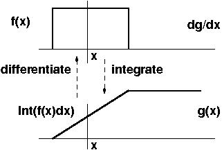
Informally, the derivative y'(x) gives the slope of function y(x).
Likewise the integral (say from 0 to t) of y(x) measures the area
under the curve y(x).
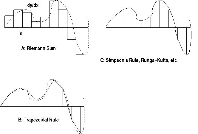
The picture says it all:

The integral is the limit of a sum; it's a continuous
sum of infinitesimal, same as a derivative is an infinitesimal
difference.
In computing, we don't have infinitesimals nor continuous numbers:
every "integral" is really a summation (unless it's a symbolic
integral).
DE Solutions: Integration
If we know y'(x) = g(x), then if we integrate both sides, we get an
equation y(x) = G(x), where G is the integral of g.
Hence "Solving a DE" = "Integrating a DE" and "Numerical Integration"
is approximate computer solution.
Examples:
d(axn)/dt = naxn-1, so
y' = naxn-1 means y = axn +C.
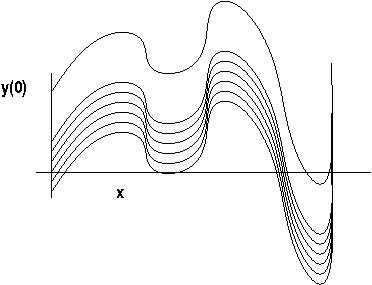
Here, C is a constant of integration. Generally DE solutions are families
of equations.

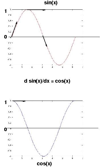
sin(x)' = cos(x), cos(x)' = -sin(x)
d eax/dt = aeax, so y' = ay means y(t) =
Ceat.
Families of Solutions
As written a DE has a family of related solutions. For example,
If y'(x) = 20x3 + 14 x, then
y(x) = 5x4 + 7 x2 + C, where
C is a "constant of integration".

Can specify one of a family of solutions by specifying Boundary
Conditions (values of variables and their derivatives) it must also satisfy.
We'll only have Initial Conditions (hence "Initial Value Problems").
Another case we won't explore
is the one where we need to
specify what happens at "both ends" of the solution for instance
("Boundary
Value Problems"). E.g. What's the distrbution of temperature in a
metal plate
whose periphery is kept cooled to a constant temp (the boundary
condition) but which is being heated in the middle?
Definitions
Ordinary and Partial DEs: ordinary d/dt and partial ∂ / ∂ t
derivatives.
Order of DE: order of highest derivative appearing in it.
An nth order DE can be expressed as a system of n 1st-order DEs, as
we'll see.
Linear and Nonlinear DEs: Linear DE in y is a sum of weighted
y-derivatives of different orders set equal to 0:
a(x)y'' +b(x)y' + c(x) y + d(x) = 0
Nonlinear has more complex relations between the derivatives, like
a(x)y''y +b(x)(y'2) + c(x) √ y + d(x) = 0
Linear constant coefficient equations have solutions in exponentials
(decays, explosions, and sines)
ay'' +by' + cy + d = 0
Homogeneous and Nonhomogeneous: Hom looks like
a(x)y'' +b(x)y' + c(x) y = 0
Nonhom:
a(x)y'' +b(x)y' + c(x) y = -d(x)
Homogeneous can be a steady state solution (no 'driving force' from
outside). Any solution to a DE can have the homogeneous soln added to
it and stay a soln.
Higher Order ODEs, Systems of 1st Order ODEs
Invent new variables (say u1, u2, u3,
etc.) so that the first one is y' the derivative of y, the second is the
derivative of the first (y''), etc. So if
y''' + g(x)y'' +r(x)y' + s(x)y = t(x),
then we must have
u1(x) = y'
u2(x) = u1' = y''
u3(x)= u2' = y''' = t(x) -s(x)y -r(x)u1 -
g(x)u2.
There is a rather nicer (to my mind) matrix form of this, also given in the
pdf reading:
Informal DE Intro.
In Matrix Form
y''' + g(x)y'' + r(x) y' + s(x)y = t(x)
   |y  | | 0     1     0   ||y  | |0   |
d  |   | |                 ||   | |    |
-- |y' |=| 0     0     1   ||y' |+|0   |
dx |   | |                 ||   | |    |
   |y''| |-s(x) -r(x) -g(x)||y''| |t(x)|
Higher Order ODEs, Systems of 1st Order ODEs
Another example of a nonlinear system of three first order DEs (The Lorenz
Attractor):
x' = 10(x-y)
y' = -xz +28x -y
z' = xy -8z/3
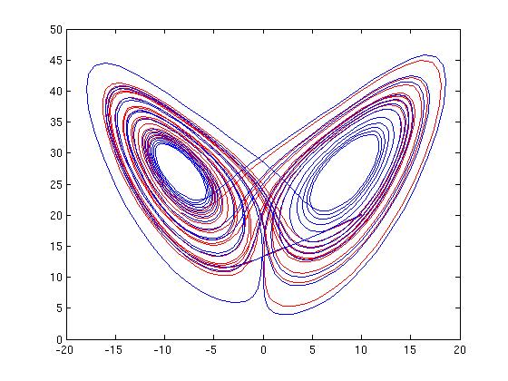
Which has a "chaotic" regime, solutions as below:
red and blue solns from almost identical initial conditions.

Final word. All the equations we feed Matlab to get our ODE
solving done will look like
y' = f(y,x).
Numerical Integration: The Idea
For Initial Boundary Value Problem. Assume know y(0), the given
initial condition. But y'(x) tells you how much to change y for a
small step in x. So step a bit dx along x and use y' to get a new
value
for y: in fact, just iteratively set y(x+dx) = y(x) + (dx)y'.
That's ALL THERE IS!! Everything else is just bells and
whistles.

Add Rectangles, Trapezoids, or small areas from higher-order approximations:
Trapezoidal Rule, Simpson's Rule, Runga-Kutta, Predictor-Corrector...
All doing the same idea with varying degrees of accuracy, speed,
flexibility, efficiency.
Stiffness: solutions at hugely different timescales means intelligent
and varying choice of step size is needed (e.g. Matlab's ode45 and
ode45s).
ODEs in Matlab: Example I
Insult Warning! This stuff is simple!
Here's an example (PLENTY more out there in
Matlab documentation , etc.
Lorenz Attractor:
x' = 10(x-w)
w' = -xz +28x -w
z' = xw -8z/3
First Matlab needs a function that computes a column vector
of derivatives
y' = f(t,y)
with one row
for each of the unknowns y(i) in our equation. This
function takes two
arguments, a scalar 'time' t and a vector of of unknown
variables.
Here we have
y(1) = x, y(2) = w, and y(3) = z. We write a function that looks like this:
function dy = lorenz(t, y)
%Lorenz Attractor. t a scalar,
% y a vector of y's.
%dy returned as a column vector of dy's
% y(1), y(2) ... are the x,y,z...
dy = zeros(3,1);
dy(1) = 10*(y(2) - y(1));
dy(2) = - y(1)*y(3) + 28*y(1) - y(2);
dy(3) = y(1)*y(2)-(8/3)*y(3);
end
The equations are implicitly parameterized by time, which steps along
according to a timespan parameter vector (next slide).
Running Matlab ODE Solver
Now we've got our derivatives function, which computes the
current derivative value from the
values of lower-order derivatives and the time.
We want to pass this function to another function as argument. As usual
with imperative languages, we'll pass a pointer, or a
handle for this function, given by Matlab's @ operator: E.g., either the bare
@lorenz
Or we can give it a name:
lorenzhandle = @lorenz
We need to
specify the time interval to be
covered by the integration. The documentation says it can be a 2-vector
[start, finish]
or an N-vector like
timespan = linspace(start, finish,1000)
With the 2-vector, Matlab makes up the spacing: the N-vector
provides explicit times (not necessarily evenly spaced).
We also need a (row or column) vector of initial conditions for the
system.
E.g. for Lorenz,
let's start at some point in space (x(0), y(0), z(0)) = [10, -10,
20] . Let's run for 20 time-units divided up into 1500 steps. We
also must be able to spell ode23, the simplest and cheapest
of Matlab's many ODE solvers.
We expect the output
to be a column vector of times (the same as our timespan input, or
made up by Matlab to lie between our start and end time), and
values of the function (and any lower-order derivatives it computes
while integrating). OK, we're off!...
%Script to Run Lorenz
lorenzhandle = @lorenz;
y0 = [10, -10, 20]; % initial conditions
%next specify 1500 instants
timespan = linspace(0, 20, 1500);
% ** boom **
[T,Y] = ode23 (lorenzhandle,timespan, y0);
% ** it's over! **
plot(Y(:,1),Y(:,3), 'r');
hold on
% new initial conditions close to previous
y0 = [10, -10, 20.1];
[T,Y] = ode23 (lorenzhandle,timespan, y0);
%BUT big difference in the two solns
plot(Y(:,1),Y(:,3), 'b');
The Plot: Y(1) versus Y(3) (X vs Z)

Matlab ODE Solver: Example II
In a vacuum, a falling body accelerates due the force of gravity.
On earth, the acceleration due to gravity is called
g = 9.8m/sec2.
Let's plot the velocity and position of a ball (in a vacuum) acted on
by
gravity. We can start the ball at what ever height and velocity we
want...
throwing it up sounds interesting (and is like the ballistics assignment).
The equation governing y as a function of time is, assuming y measures height,
y'' = -g
We put that into our favorite matrix form this way.
d  |y  |   | 0  1| |y  |   |0    |
-- |   | = |     | |   | + |     |
dx |y' |   | 0  0| |y' |   |-9.8 |
dy/dx = y'
d2 y / d y2 = y'' = -9.8
So our derivatives function in Matlab is this:
function dy = ball(t,y)
dy = zeros(2,1);
dy(1) = y(2); %dy/dx = y'
dy(2) = -9.8; %d2 y / d y2 = y'' = -9.8
end
We now get to choose a start and finish time and initial
conditions. May as well start at zero time and altitude.
Let's start the ball off with an upward velocity of 100m/sec.
% script
ballhandle = @ball;
tspan = [0 20]; % [start finish] (seconds)
y0 = [0 100]; % [ y y'] initial
[T Y] = ode23(ballhandle, tspan, y0); %boom
....
>> [T Y]
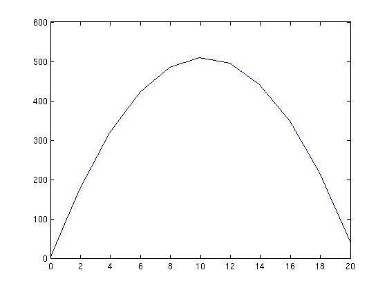
>> plot(T,Y(:,1))
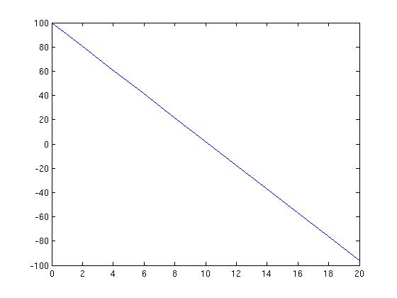
>> plot(T,Y(:,2))
The Output Matrices and Plots
Notice Matlab starts out with small dt time steps, but
grows confident and starts moving along by 2 each step, which actually
leave us with a rather un-smooth graph...
      T         Y       VEL
         0         0  100.0000
    0.0000    0.0001  100.0000
    0.0000    0.0005  100.0000
    0.0000    0.0025   99.9998
    0.0001    0.0125   99.9988
    0.0006    0.0625   99.9939
    0.0031    0.3124   99.9694
    0.0156    1.5613   99.8469
    0.0781    7.7826   99.2344
    0.3906   38.3148   96.1719
    1.9531  176.6205   80.8594
    3.9531  318.7392   61.2594
    5.9531  421.6580   41.6594
    7.9531  485.3767   22.0594
    9.9531  509.8955    2.4594
   11.9531  495.2142  -17.1406
   13.9531  441.3330  -36.7406
   15.9531  348.2517  -56.3406
   17.9531  215.9705  -75.9406
   20.0000   40.0000  -96.0000
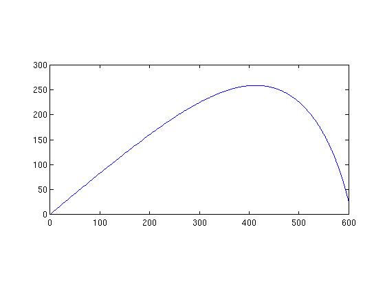
Velocity Below

Height Below

Simulations and Fun
Simulations are great fun, since we get to play around with the
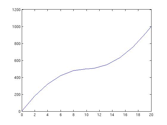
rules. Suppose the force of gravity were a nice even 10, and
that its direction is reversed 10
seconds into the ball's flight?
function dy = gball(t,y)
if t<10
g = -10;
else
g = 10;
end
dy = zeros(2,1);
dy(1) = y(2);
dy(2) = g;
end
and
Height Below

Last Words
Our goals were:
- to demystify DEs
- to encourage you as always to READ
(texts, papers, documentation, websites, tutorials) FOR YOURSELVES
- to show easy examples of solving initial-value problems with
higher-order ODEs and systems of ODEs in Matlab.

Trajectory of human head launched at 40 degrees of elevation into enemy
redoubt.
Flight took about 15 seconds. Distance unit is the meter (about 3 feet for
you Angles and Saxons).

Last update: 04/22/2011: RN
